
Note: This notebook reproduces all quantitative results of the paper step by step.
Reproducing the study step by step#
Storage in Long-Term Energy Planning Models with Temporal Aggregation: Best Practices and Algorithms Bruno Borba, Md Eliasinul Islam, Taco Niet — Environmental Research Communications (manuscript ERC-105849)
This notebook regenerates every quantitative result of the paper from the inputs in this repository. Each model run calls workflow/main.py unchanged, so the notebook exercises the same code path that produced the published numbers.
Step |
Paper section |
What it does |
Default |
Approx. cost* |
|---|---|---|---|---|
1 |
3.4 |
Environment check against the stated versions |
on |
seconds |
2 |
3.3, Table 3 |
Model inputs and time series (Figures 4–5) |
on |
seconds |
3 |
3.2 |
Representative-day clustering; determinism and multi-seed robustness |
on |
~30 s |
4 |
4.1 |
Independent hand-calculated SoC verification |
on |
~10 s |
5 |
— |
Reproduction check: k4h1 for WND, SOL, HYD against the archived results |
on |
~1 min |
6 |
4.1 |
Full-year hourly benchmarks k365h1 (Figure 6, Table S1) |
off |
~15 min per resource, ~12 GB RAM (Novo) |
7 |
4.2–4.3 |
108 aggregated configurations × 3 resources (Figures 7–8, Tables S2–S4) |
off |
2–4 h (0.8 h solver time), ≤ 3 GB RAM |
8 |
4.2 |
Table 4 and cost-error curves |
on (archive or fresh) |
seconds |
9 |
4.4 |
Binding-capacity stress test, 0.2 kW·yr (Figures 9–10) |
off (archive stats on) |
~20 min per resource |
10 |
4.3 |
SoC fidelity metrics: MAE, RMSE, Pearson, rainflow (Figure 8) |
on (archive) |
seconds |
11 |
3.2 |
Seed sensitivity of system cost |
off |
~10 min |
*Measured with GLPK 5.0 on an Intel Core i7 / 16 GB machine (archived run logs).
Name mapping. The formulation called Novo in the paper is implemented in Model_Cluster; Niet, Welsch and Kotzur map to Model_Niet, Model_Welsch and Model_Kotzur.
Scenario labels. k20h1HYD = 20 representative days, 1-hour intra-day blocks, hydro-dominated system. The suffix _limited marks the stress test.
0. Setup#
Set the switches below to run the heavy steps. Everything else reads either fresh results (folder results/) or the archived results that accompany the paper.
[23]:
from pathlib import Path
import sys, json
import numpy as np, pandas as pd
import matplotlib.pyplot as plt

REPO = Path.cwd() if (Path.cwd() / 'workflow').is_dir() else Path.cwd().parent   # repository root or notebooks/
assert (REPO / 'workflow' / 'main.py').exists(), 'Start Jupyter from the repository root or from notebooks/.'
sys.path.insert(0, str(REPO))
import src.reproduce as rp

# ---- switches for the heavy steps -------------------------------------------------------
RUN_REPRODUCTION_CHECK = True    # step 5: k4h1 x 3 resources (~1 min)
RUN_BENCHMARK          = True   # step 6: k365h1 x 3 resources (needs ~12 GB RAM for Novo)
RUN_SWEEP              = True   # step 7: full grid (2-4 h); see SWEEP_* below
RUN_STRESS             = True   # step 9: k365h1 WND and SOL with a 0.2 kW.yr cap
RUN_SEED_COSTS         = True   # step 11: optimisation under alternative k-means seeds

SWEEP_RESOURCES = ['WND', 'SOL', 'HYD']
SWEEP_K         = rp.K_VALUES          # [2..10, 20..100]
SWEEP_H         = rp.H_VALUES          # [1, 2, 4, 6, 8, 12]
FRESH = REPO / 'results'               # fresh runs are written here

# ---- archived results of the published study --------------------------------------------
PUBLISHED = REPO / 'data' / 'published_results'           # tracked subset (tables + key trajectories)
FULL_ARCHIVE = REPO / 'data' / 'full_archive'             # optional: full archive (Zenodo), all CSVs
ARCH_MAIN = FULL_ARCHIVE / 'Results_Demand_Variation' if FULL_ARCHIVE.exists() else PUBLISHED / 'main'
ARCH_LIM  = FULL_ARCHIVE / 'Results_Limited' if FULL_ARCHIVE.exists() else PUBLISHED / 'limited'
archive = rp.load_results(ARCH_MAIN / 'Simulation_Results.xlsx')
archive_lim = rp.load_results(ARCH_LIM / 'Simulation_Results.xlsx')
print(f'Archive: {len(archive)} rows, {archive.Scenario.nunique()} scenarios  ({ARCH_MAIN.relative_to(REPO)})')
plt.rcParams.update({'figure.dpi': 110, 'axes.grid': True, 'grid.alpha': .3})
COLORS = {'Niet': '#d62728', 'Welsch': '#8c564b', 'Kotzur': '#1f77b4', 'Novo': '#2ca02c'}
Archive: 1308 rows, 327 scenarios (data/full_archive/Results_Demand_Variation)
1. Computational environment (Section 3.4)#
Set up with conda env create -f env/environment-crossplatform.yml (GLPK 5.0 from conda-forge, also on Windows). The paper reports GLPK 5.0, Python 3.13.5, otoole 1.1.5 and scikit-learn 1.7.1. Solver version affects runtimes; scikit-learn version affects clustering (before 1.4, KMeans defaulted to n_init=10; the code now sets n_init=1 explicitly).
[24]:
env = rp.check_environment()
env
[24]:
| component | manuscript | installed | status | |
|---|---|---|---|---|
| 0 | python | 3.13.5 | 3.13.5 | match |
| 1 | glpsol | 5.0 | 5.0 | match |
| 2 | otoole | 1.1.5 | 1.1.5 | match |
| 3 | scikit-learn | 1.7.1 | 1.7.1 | match |
| 4 | pandas | 2.2.3 | 2.2.3 | match |
| 5 | numpy | 2.3.1 | 2.3.1 | match |
2. Model inputs (Section 3.3, Table 3; Figures 4–5)#
A single-node system: one VRE technology (label WINDPOWER for all three resources; only its capacity-factor profile changes), one battery and an electricity demand. The values below are read directly from data/system/ and the otoole defaults, i.e. what the solver actually sees.
Note. Annual demand (20) and the VRE variable cost (20) are not listed in Table 3 of the paper, but both change total cost.
[25]:
import yaml
def csv_val(name, **flt):
    d = pd.read_csv(REPO / 'data' / 'system' / f'{name}.csv')
    for k, v in flt.items(): d = d[d[k] == v]
    return d['VALUE'].iloc[0] if len(d) else None
otc = yaml.safe_load(open(REPO / 'models' / 'Model_Niet' / 'otoole_config_Niet.yaml'))
cfg = yaml.safe_load(open(REPO / 'config' / 'config.yaml'))
default = lambda p: otc[p]['default']
table3 = pd.DataFrame([
    ('VRE capital cost', csv_val('CapitalCost', TECHNOLOGY='WINDPOWER'), 'data/system/CapitalCost.csv'),
    ('VRE variable cost', csv_val('VariableCost', TECHNOLOGY='WINDPOWER'), 'data/system/VariableCost.csv'),
    ('Storage capital cost (per kW.yr)', default('CapitalCostStorage'), 'otoole default'),
    ('Storage charge input ratio (1/round-trip eff.)', csv_val('InputActivityRatio', TECHNOLOGY='BATTERY_STORAGE'), 'data/system/InputActivityRatio.csv'),
    ('Storage variable cost', default('VariableCost'), 'otoole default (battery not listed in VariableCost.csv)'),
    ('Annual electricity demand', csv_val('SpecifiedAnnualDemand'), 'data/system/SpecifiedAnnualDemand.csv'),
    ('Residual storage capacity (kW.yr)', cfg['ResidualStorageCapacity'], 'config/config.yaml'),
    ('Minimum storage charge', default('MinStorageCharge'), 'otoole default'),
    ('Discount rate', default('DiscountRate'), 'otoole default'),
    ('Operational life (years)', default('OperationalLife'), 'otoole default'),
    ('Storage energy cap, unconstrained runs (kW.yr)', rp.UNCONSTRAINED_CAP, 'reproduce.py'),
    ('Storage energy cap, stress test (kW.yr)', rp.STRESS_CAP, 'reproduce.py'),
], columns=['Parameter', 'Value', 'Source'])
table3
[25]:
| Parameter | Value | Source | |
|---|---|---|---|
| 0 | VRE capital cost | 1200.00 | data/system/CapitalCost.csv |
| 1 | VRE variable cost | 20.00 | data/system/VariableCost.csv |
| 2 | Storage capital cost (per kW.yr) | 1000.00 | otoole default |
| 3 | Storage charge input ratio (1/round-trip eff.) | 1.25 | data/system/InputActivityRatio.csv |
| 4 | Storage variable cost | 20.00 | otoole default (battery not listed in Variable... |
| 5 | Annual electricity demand | 20.00 | data/system/SpecifiedAnnualDemand.csv |
| 6 | Residual storage capacity (kW.yr) | 0.05 | config/config.yaml |
| 7 | Minimum storage charge | 0.00 | otoole default |
| 8 | Discount rate | 0.05 | otoole default |
| 9 | Operational life (years) | 1.00 | otoole default |
| 10 | Storage energy cap, unconstrained runs (kW.yr) | 1000.00 | reproduce.py |
| 11 | Storage energy cap, stress test (kW.yr) | 0.20 | reproduce.py |
[26]:
D = REPO / 'data' / 'timeseries'
cf = {r: pd.read_csv(D / f)['VALUE'].to_numpy() for r, f in rp.RESOURCES.items()}
dem = pd.read_csv(D / rp.DEMAND_PROFILE)['VALUE'].to_numpy()
fig, ax = plt.subplots(1, 2, figsize=(12, 3.6))
for r, v in cf.items():
    ax[0].plot(v.reshape(365, 24).mean(1), lw=.8, label=r)
    ax[1].plot(v.reshape(365, 24).mean(0), marker='o', ms=3, label=r)
ax[0].set(title='Daily mean capacity factor', xlabel='Day of year', ylabel='CF (-)')
ax[1].set(title='Average diurnal profile', xlabel='Hour of day', ylabel='CF (-)')
ax[0].legend(); plt.tight_layout(); plt.show()
fig, ax = plt.subplots(figsize=(12, 2.8))
ax.plot(dem.reshape(365, 24).sum(1), color='k', lw=.8)
ax.set(title='Demand profile: daily share of annual demand', xlabel='Day of year', ylabel='share (-)')
plt.tight_layout(); plt.show()
print({r: dict(mean=v.mean().round(3), min=v.min().round(3), max=v.max().round(3)) for r, v in cf.items()},
      '| demand profile sums to', dem.sum().round(6))
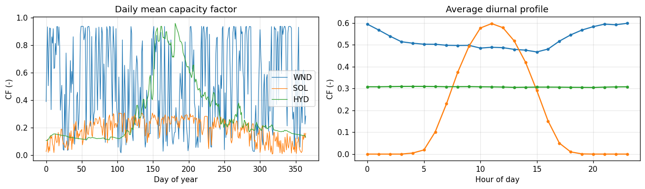
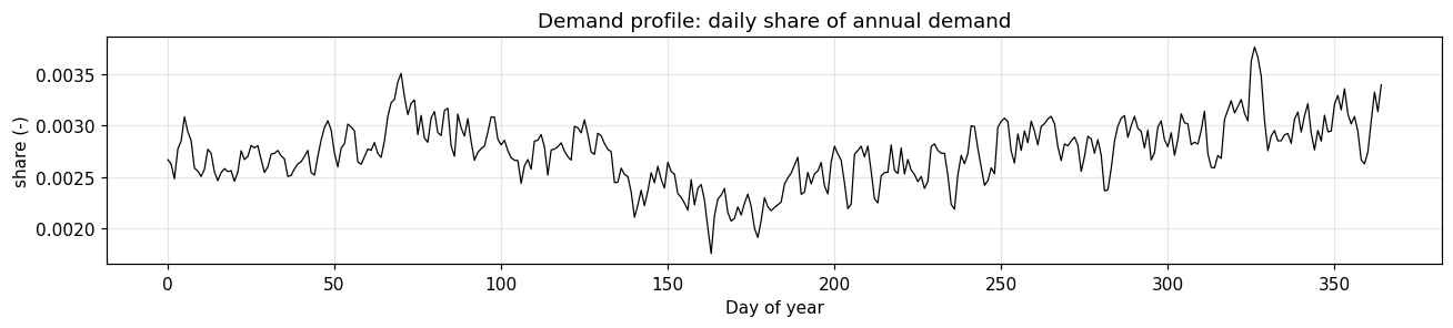
{'WND': {'mean': np.float64(0.524), 'min': np.float64(0.01), 'max': np.float64(0.939)}, 'SOL': {'mean': np.float64(0.184), 'min': np.float64(0.0), 'max': np.float64(0.941)}, 'HYD': {'mean': np.float64(0.307), 'min': np.float64(0.107), 'max': np.float64(1.0)}} | demand profile sums to 1.0
3. Representative days (Section 3.2)#
Each day is a 48-dimensional vector (24 min–max-scaled capacity factors and 24 scaled demand values). k-means (scikit-learn, k-means++ initialisation, n_init = 1, random_state = 0) partitions the 365 days, and the day closest to each centroid becomes the representative day. All four formulations receive the same clustering.
[27]:
rep, seq = rp.clustering('WND', 4)
rep2, seq2 = rp.clustering('WND', 4)
print('Representative days (WND, k=4):', rep)
print('Days represented by each:', {d: seq.count(d) for d in rep})
print('Deterministic for a fixed seed:', rep == rep2 and seq == seq2)
Representative days (WND, k=4): [66, 190, 257, 296]
Days represented by each: {66: 44, 190: 84, 257: 128, 296: 109}
Deterministic for a fixed seed: True
3.1 Multi-seed robustness#
The clustering is repeated with seeds 1–9 and compared with seed 0:
ARI: adjusted Rand index of the day partition (1 = identical partition up to relabelling; 0 = chance level).
day agreement: share of days assigned to the same representative day as with seed 0 (stricter, because two seeds can find the same cluster but a different medoid day).
same representative days: whether the selected set of days is identical.
[ ]:
seeds = rp.seed_robustness()
summary_seed = (seeds.groupby('k')[['ARI', 'day_agreement', 'same_rep_days']].mean()
                     .rename(columns={'same_rep_days': 'share identical rep-day sets'}))
display(summary_seed.round(3).T)
print('Over all resources, k and seeds: mean ARI = %.3f (min %.3f); mean day agreement = %.3f; '
      'identical representative-day sets in %d of %d comparisons.'
      % (seeds.ARI.mean(), seeds.ARI.min(), seeds.day_agreement.mean(), seeds.same_rep_days.sum(), len(seeds)))
stats = seeds.groupby(['resource', 'k']).ARI.agg(['mean', 'min', 'max'])
fig, axs = plt.subplots(1, 3, figsize=(12, 3.2), sharex=True, sharey=True)
for ax, (r, m), c in zip(axs, stats.groupby(level='resource'), ['C0', 'C1', 'C2']):
    m = m.droplevel('resource')
    ax.fill_between(m.index, m['min'], m['max'], color=c, alpha=.2, lw=0, label='min–max')
    ax.plot(m.index, m['mean'], '-o', color=c, ms=3.5, lw=1.5, label='mean')
    ax.axhline(1, color='0.5', ls='--', lw=.8)
    ax.set_title(r, loc='left', fontweight='bold')
    ax.set_xlabel('Representative days $k$')
    ax.spines[['top', 'right']].set_visible(False)
axs[0].set(xscale='log', ylim=(0, 1.05), ylabel='ARI vs. seed 0')
axs[0].set_xticks([2, 5, 10, 20, 50, 100], labels=[2, 5, 10, 20, 50, 100]); axs[0].minorticks_off()
axs[0].legend(frameon=False, loc='lower left')
fig.suptitle('Clustering stability across seeds 1–9', x=0.01, ha='left')
plt.tight_layout(); plt.show()
Interpretation/Caption: Stability of the representative-day selection across k-means seeds. For each scenario and number of representative days k, nine alternative seeds are compared with the reference seed on two measures: agreement in how days are grouped into clusters (adjusted Rand index, solid) and agreement in which calendar day is selected to represent each cluster (dashed). Lines are means over the nine seeds; shaded bands span the minimum and maximum.
Alternative views#
all three metrics side by side; (b) heatmaps with exact values; (c) every seed as a dot, so the spread is visible;
ARI against day agreement: points well below the diagonal found nearly the same clusters but picked a different representative (medoid) day.
[ ]:
# Alternative views of the same `seeds` table (the plot above is kept as is)
COL = {'WND': '#0072B2', 'SOL': '#E69F00', 'HYD': '#009E73'}           # Okabe-Ito, colour-blind safe
ks = sorted(seeds.k.unique()); xi = {k: i for i, k in enumerate(ks)}    # categorical k axis (even spacing)
metrics = {'ARI': 'ARI vs seed 0', 'day_agreement': 'Day agreement', 'same_rep_days': 'Identical rep-day set'}
agg = seeds.groupby(['resource', 'k'])[list(metrics)].mean()

# (a) Small multiples: the three metrics side by side, k on an evenly spaced categorical axis
fig, axs = plt.subplots(1, 3, figsize=(12, 3.2), sharex=True, sharey=True)
for ax, (col, lab) in zip(axs, metrics.items()):
    for r, c in COL.items():
        m = agg.loc[r, col]
        ax.plot([xi[k] for k in m.index], m.values, marker='o', ms=4, lw=1.8, color=c, label=r)
    ax.set(title=lab, ylim=(-0.03, 1.03), xticks=range(len(ks)))
    ax.set_xticklabels(ks, fontsize=7); ax.grid(axis='y', alpha=.3); ax.spines[['top', 'right']].set_visible(False)
axs[0].set_ylabel('Mean over seeds 1–9'); axs[1].set_xlabel('Representative days k')
axs[0].legend(frameon=False, fontsize=8)
fig.suptitle('(a) Three stability metrics vs seed 0', x=0.01, ha='left'); plt.tight_layout(); plt.show()

# (b) Heatmaps: resource x k, mean ARI and mean day agreement, annotated
fig, axs = plt.subplots(2, 1, figsize=(12, 3.6), sharex=True)
for ax, col in zip(axs, ['ARI', 'day_agreement']):
    h = agg[col].unstack('k').loc[list(COL)]
    im = ax.imshow(h.values, cmap='Blues', vmin=0, vmax=1, aspect='auto')
    for (i, j), v in np.ndenumerate(h.values):
        ax.text(j, i, f'{v:.2f}', ha='center', va='center', fontsize=7, color='white' if v > .6 else 'black')
    ax.set(yticks=range(len(h)), yticklabels=h.index, xticks=range(len(ks)), xticklabels=ks)
    ax.set_ylabel(metrics[col], rotation=0, ha='right', va='center')
axs[-1].set_xlabel('Representative days k')
fig.colorbar(im, ax=axs, fraction=.02, pad=.01)
fig.suptitle('(b) Mean stability by resource and k', x=0.01, ha='left'); plt.show()

# (c) Every seed as a dot: one panel per resource, shows the spread rather than a min-max band
fig, axs = plt.subplots(1, 3, figsize=(12, 3.2), sharey=True)
rng = np.random.default_rng(0)
for ax, (r, c) in zip(axs, COL.items()):
    g = seeds[seeds.resource == r]
    x = g.k.map(xi) + rng.uniform(-.18, .18, len(g))
    ax.scatter(x, g.ARI, s=12, color=c, alpha=.55, lw=0)
    m = g.groupby('k').ARI.median()
    ax.scatter([xi[k] for k in m.index], m.values, marker='_', s=180, color='k', lw=1.5, label='median')
    ax.set(title=r, xticks=range(len(ks)), ylim=(0.3, 1.02)); ax.set_xticklabels(ks, fontsize=7)
    ax.grid(axis='y', alpha=.3); ax.spines[['top', 'right']].set_visible(False)
axs[0].set_ylabel('ARI vs seed 0'); axs[1].set_xlabel('Representative days k'); axs[0].legend(frameon=False, fontsize=8)
fig.suptitle('(c) ARI of each seed (dots) and median (bar)', x=0.01, ha='left'); plt.tight_layout(); plt.show()

# (d) Partition vs medoid: ARI against day agreement; points far below the diagonal found the same
#     clusters but picked a different representative day
fig, ax = plt.subplots(figsize=(5.2, 4.4))
for r, c in COL.items():
    g = seeds[seeds.resource == r]
    ax.scatter(g.ARI, g.day_agreement, s=8 + 0.6 * g.k, color=c, alpha=.5, lw=0, label=r)
ax.plot([0, 1], [0, 1], color='grey', lw=1, ls='--')
ax.set(xlim=(0.3, 1.02), ylim=(-0.03, 1.03), xlabel='ARI (partition)', ylabel='Day agreement (same medoid)')
ax.legend(frameon=False, title='marker size ∝ k', fontsize=8, title_fontsize=8)
ax.spines[['top', 'right']].set_visible(False)
ax.set_title('(d) Same clusters, different representative day?', loc='left', fontsize=10)
plt.tight_layout(); plt.show()
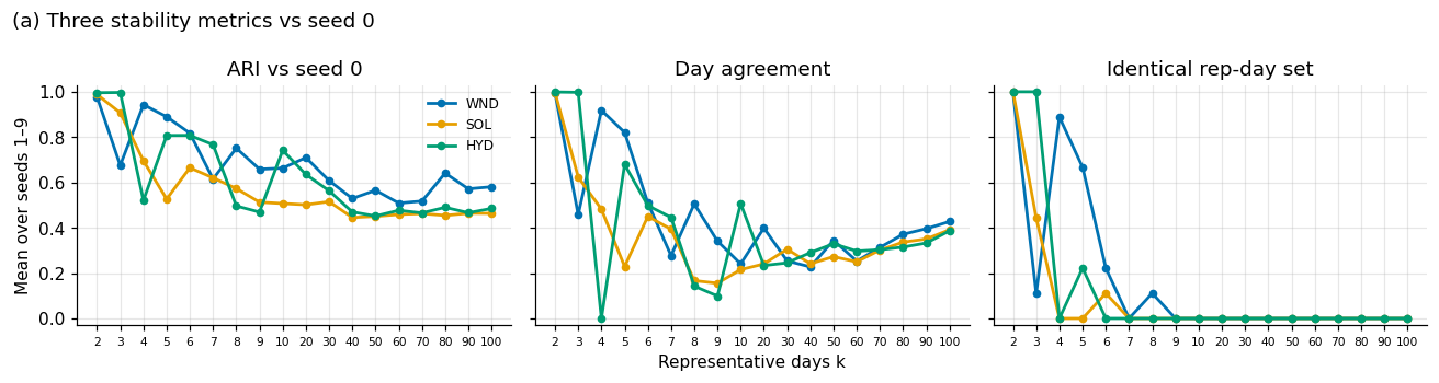
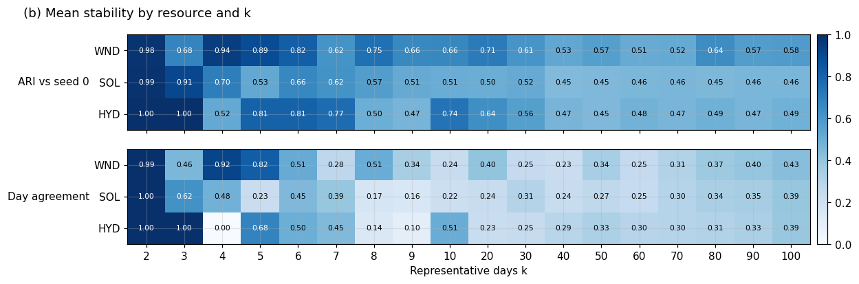
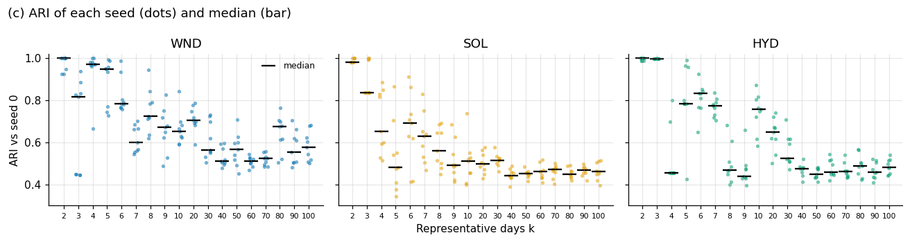
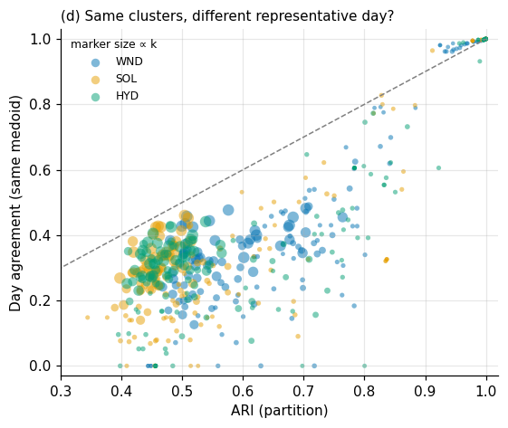
Interpretation. A fixed seed makes the comparison between formulations fair (identical inputs), but it does not make the reported error levels seed-independent. Whether the different clusterings change cost errors and the ranking of formulations is tested in step 11.
4. Independent SoC verification (Section 4.1)#
Four days A–B–A–B, four 6-h blocks per day, no losses, fixed capacities. Each occurrence of A adds 6 MWh and each B removes 6 MWh. The hand-calculated SoC sequence of each formulation (validation/soc/independent_reference.csv) is compared with the model output; for Kotzur and Welsch the existing intraday reconstructions are also checked.
[ ]:
soc_val = rp.run_soc_validation()
display(soc_val)
assert soc_val[['Max_native_error_MWh', 'Max_reconstructed_error_MWh']].fillna(0).abs().max().max() < 1e-6
print('All native and reconstructed SoC values match the hand calculation.')
| Formulation | Native_points | Max_native_error_MWh | Max_reconstructed_error_MWh | |
|---|---|---|---|---|
| 0 | Niet | 8 | 0.0 | NaN |
| 1 | Welsch | 2 | 0.0 | 0.0 |
| 2 | Kotzur | 4 | 0.0 | 0.0 |
| 3 | Novo | 16 | 0.0 | NaN |
All native and reconstructed SoC values match the hand calculation.
5. Reproduction check against the archived results#
Runs k4h1 for the three resources (12 model solves) and compares cost, VRE capacity and storage capacity with the archived study results. Agreement to solver precision confirms that the inputs and code in this repository are those behind the paper.
[ ]:
if RUN_REPRODUCTION_CHECK:
    fresh = pd.concat([rp.run_case(r, 4, 1, results_dir=FRESH, verbose=True) for r in ['WND', 'SOL', 'HYD']])
    chk = rp.compare_to_archive(fresh, archive)
    display(chk[['Scenario', 'Model', 'Total cost (new)', 'Total cost (archive)', 'Total cost rel. diff',
                 'Storage Capacity rel. diff', 'Power Capacity rel. diff']])
    worst = chk.filter(like='rel. diff').max().max()
    print(f'Largest relative difference: {worst:.2e}')
    assert worst < 1e-6, 'Fresh results differ from the archive'
k4h1WND: done in 9.0 s
k4h1SOL: done in 8.9 s
k4h1HYD: done in 8.9 s
| Scenario | Model | Total cost (new) | Total cost (archive) | Total cost rel. diff | Storage Capacity rel. diff | Power Capacity rel. diff | |
|---|---|---|---|---|---|---|---|
| 0 | k4h1WND | Model_Cluster | 50762.64310 | 50762.64310 | 0.0 | 0.000000e+00 | 2.437632e-15 |
| 1 | k4h1WND | Model_Kotzur | 50762.64310 | 50762.64310 | 0.0 | 0.000000e+00 | 0.000000e+00 |
| 2 | k4h1WND | Model_Niet | 56593.84319 | 56593.84319 | 0.0 | 2.821359e-15 | 2.437634e-15 |
| 3 | k4h1WND | Model_Welsch | 56203.53786 | 56203.53786 | 0.0 | 1.223122e-14 | 2.193871e-14 |
| 4 | k4h1SOL | Model_Cluster | 152451.86590 | 152451.86590 | 0.0 | 6.983842e-15 | 0.000000e+00 |
| 5 | k4h1SOL | Model_Kotzur | 152431.26640 | 152431.26640 | 0.0 | 4.540588e-15 | 0.000000e+00 |
| 6 | k4h1SOL | Model_Niet | 156668.35310 | 156668.35310 | 0.0 | 2.495922e-15 | 0.000000e+00 |
| 7 | k4h1SOL | Model_Welsch | 154447.48990 | 154447.48990 | 0.0 | 4.427132e-14 | 4.077409e-14 |
| 8 | k4h1HYD | Model_Cluster | 82299.83452 | 82299.83452 | 0.0 | 2.200870e-14 | 4.225193e-14 |
| 9 | k4h1HYD | Model_Kotzur | 82299.83452 | 82299.83452 | 0.0 | 4.323137e-15 | 3.002675e-15 |
| 10 | k4h1HYD | Model_Niet | 82145.66355 | 82145.66355 | 0.0 | 4.639626e-15 | 3.002676e-15 |
| 11 | k4h1HYD | Model_Welsch | 82184.02944 | 82184.02944 | 0.0 | 0.000000e+00 | 1.501338e-15 |
Largest relative difference: 4.43e-14
6. Full-year hourly benchmarks (Section 4.1, Figure 6, Table S1)#
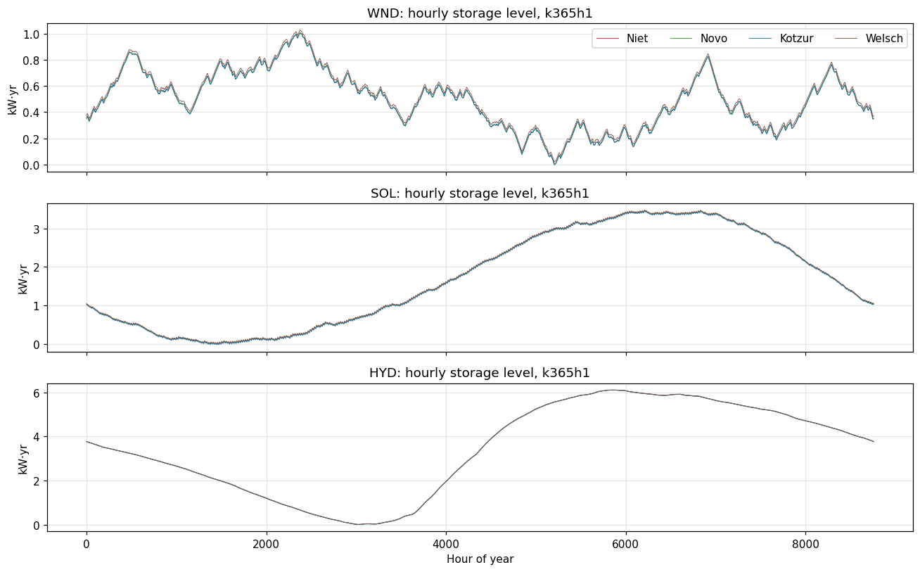
k = 365, h = 1 for each resource. At full resolution the mapping is the identity and all four formulations reduce to the same recursion, so their SoC curves coincide; this is a consistency check, not an independent validation. Novo needs about 12 GB of RAM at k365h1.
[ ]:
if RUN_BENCHMARK:
    for r in ['WND', 'SOL', 'HYD']:
        rp.run_case(r, 365, 1, results_dir=FRESH, verbose=True)

def results_source():
    # archive, with failed solves replaced by re-solved values, overridden by fresh runs
    a = archive.copy()
    failed = a['Total cost'].fillna(0) <= 0          # GLPK failure recorded as cost 0 (see Step 7)
    rerun_f = PUBLISHED / 'corrections' / 'welsch_reruns.xlsx'
    if failed.any() and rerun_f.exists():
        rr = rp.load_results(rerun_f)
        a = pd.concat([a[~failed], rr.assign(source='re-solved')], ignore_index=True)
    else:
        a = a[~failed]
    a['source'] = a.get('source', pd.Series(index=a.index, dtype=object)).fillna('archive')
    if (FRESH / 'Simulation_Results.xlsx').exists():
        f = rp.load_results(FRESH / 'Simulation_Results.xlsx')
        f = f[~f.Scenario.str.contains(r'_s\d+$')]
        key = a.Scenario + a.Model
        a = a[~key.isin(f.Scenario + f.Model)]
        a = pd.concat([a, f.assign(source='fresh')], ignore_index=True)
    return a

res = results_source()
bench = res[(res.k == 365) & (res.h == 1)]
display(bench[['resource', 'formulation', 'Total cost', 'Power Capacity', 'Storage Capacity',
               'total_time_s', 'memory_MB', 'source']].sort_values(['resource', 'formulation']))
spread = bench.groupby('resource').agg(cost_spread_pct=('Total cost', lambda x: 100 * (x.max() - x.min()) / x.min()),
                                       cap_spread=('Storage Capacity', lambda x: x.max() - x.min()))
display(spread.round(3))
| resource | formulation | Total cost | Power Capacity | Storage Capacity | total_time_s | memory_MB | source | |
|---|---|---|---|---|---|---|---|---|
| 430 | HYD | Kotzur | 90836.46212 | 70.096498 | 6.057958 | 82.98 | 613.4 | archive |
| 431 | HYD | Niet | 90840.54802 | 70.096498 | 6.062044 | 319.63 | 193.0 | archive |
| 429 | HYD | Novo | 90840.56147 | 70.096498 | 6.062057 | 491.14 | 10814.0 | archive |
| 432 | HYD | Welsch | 90852.86695 | 70.096498 | 6.074362 | 294.54 | 1051.7 | archive |
| 1 | SOL | Kotzur | 153297.51630 | 124.180955 | 3.386068 | 61.94 | 621.3 | archive |
| 2 | SOL | Niet | 153330.27880 | 124.180955 | 3.418831 | 115.51 | 185.8 | archive |
| 0 | SOL | Novo | 153330.28640 | 124.180955 | 3.418838 | 421.55 | 12195.1 | archive |
| 3 | SOL | Welsch | 153352.63050 | 124.180955 | 3.441182 | 242.08 | 1042.0 | archive |
| 859 | WND | Kotzur | 51014.00809 | 41.159057 | 0.955107 | 156.29 | 613.4 | archive |
| 860 | WND | Niet | 51015.84985 | 41.159057 | 0.956949 | 134.68 | 193.0 | archive |
| 858 | WND | Novo | 51015.85207 | 41.159057 | 0.956951 | 427.28 | 10814.0 | archive |
| 861 | WND | Welsch | 51053.51364 | 41.159057 | 0.994612 | 256.97 | 1051.7 | archive |
| cost_spread_pct | cap_spread | |
|---|---|---|
| resource | ||
| HYD | 0.018 | 0.016 |
| SOL | 0.036 | 0.055 |
| WND | 0.077 | 0.040 |
The Table 4 note in the paper states that at full resolution the formulations agree within 0.08 % on cost and 0.03 kW·yr on capacity. The spread table above is the direct check of that sentence.
[ ]:
src_dir = FRESH if (FRESH / 'k365h1WND_Storage_Level_Model_Niet.csv').exists() else ARCH_MAIN
fig, axes = plt.subplots(3, 1, figsize=(12, 7.5), sharex=True)
for ax, r in zip(axes, ['WND', 'SOL', 'HYD']):
    for f, m in [('Niet', 'Niet'), ('Novo', 'Cluster'), ('Kotzur', 'Kotzur_intraday'), ('Welsch', 'Welsch_intraday')]:
        p = src_dir / f'k365h1{r}_Storage_Level_Model_{m}.csv'
        if p.exists():
            ax.plot(rp.read_storage(src_dir, f'k365h1{r}', m), lw=.6, color=COLORS[f], label=f)
    ax.set(ylabel='kW·yr', title=f'{r}: hourly storage level, k365h1')
axes[0].legend(ncol=4); axes[-1].set_xlabel('Hour of year'); plt.tight_layout(); plt.show()
7. Aggregated configurations (Sections 4.2–4.3)#
18 values of k × 6 block lengths h = 108 configurations per resource, each solved with all four formulations. Completed scenarios are skipped, so the cell can be interrupted and resumed. The runtime estimate below is taken from the archived logs.
[ ]:
grid = archive[(archive.k != 365) & archive.resource.isin(SWEEP_RESOURCES) & archive.k.isin(SWEEP_K) & archive.h.isin(SWEEP_H)]
print(f'Selected grid: {grid.Scenario.nunique()} scenarios, {len(grid)} solves; '
      f'archived wall time {grid.total_time_s.sum() / 3600:.1f} h, peak memory {grid.memory_MB.max() / 1024:.1f} GB')
if RUN_SWEEP:
    rp.run_grid(SWEEP_RESOURCES, SWEEP_K, SWEEP_H, results_dir=FRESH)
Selected grid: 324 scenarios, 1296 solves; archived wall time 0.8 h, peak memory 2.9 GB
7.1 Audit of the archived sweep: failed solves#
Eight archived Welsch solves report a total cost of exactly 0. GLPK’s primal simplex stopped with “unable to recover undefined or non-optimal solution”, and the original pipeline then read the result CSVs left over from the previous scenario, so the capacities in these rows are stale. src/simulation.py now detects non-optimal termination, retries with --nopresol, --dual and --exact (identical optima where tested) and never reports capacities from a failed solve. The re-solved
values are in data/published_results/corrections/welsch_reruns.xlsx and replace the failed rows in all tables below.
[ ]:
failed = archive[archive['Total cost'].fillna(0) <= 0]
display(failed[['Scenario', 'Model', 'Total cost', 'Power Capacity', 'Storage Capacity']])
rr_f = PUBLISHED / 'corrections' / 'welsch_reruns.xlsx'
if rr_f.exists():
    rr = rp.add_errors(pd.concat([rp.load_results(rr_f), archive[(archive.k == 365) & (archive.Model == 'Model_Cluster')]]))
    display(rr[rr.k != 365][['Scenario', 'Model', 'Total cost', 'Power Capacity', 'Storage Capacity', 'cost_err_pct', 'cap_err_pct']].round(3))
| Scenario | Model | Total cost | Power Capacity | Storage Capacity | |
|---|---|---|---|---|---|
| 79 | k5h1SOL | Model_Welsch | 0.0 | 115.266936 | 6.280452 |
| 127 | k7h1SOL | Model_Welsch | 0.0 | 114.010711 | 4.775415 |
| 151 | k8h1SOL | Model_Welsch | 0.0 | 118.072735 | 5.597867 |
| 511 | k4h12HYD | Model_Welsch | 0.0 | 66.258262 | 2.128255 |
| 543 | k6h2HYD | Model_Welsch | 0.0 | 69.030964 | 2.822310 |
| 555 | k6h8HYD | Model_Welsch | 0.0 | 69.022945 | 2.803670 |
| 959 | k5h4WND | Model_Welsch | 0.0 | 41.392659 | 7.357507 |
| 1015 | k7h8WND | Model_Welsch | 0.0 | 43.353997 | 6.126450 |
| Scenario | Model | Total cost | Power Capacity | Storage Capacity | cost_err_pct | cap_err_pct | |
|---|---|---|---|---|---|---|---|
| 0 | k4h12HYD | Model_Welsch | 82162.458 | 66.258 | 2.123 | -9.553 | -64.986 |
| 1 | k6h2HYD | Model_Welsch | 86178.267 | 69.023 | 2.818 | -5.132 | -53.515 |
| 2 | k6h8HYD | Model_Welsch | 86111.206 | 68.989 | 2.794 | -5.206 | -53.917 |
| 4 | k5h1SOL | Model_Welsch | 152095.499 | 122.039 | 4.758 | -0.805 | 39.157 |
| 5 | k7h1SOL | Model_Welsch | 158053.098 | 126.273 | 5.618 | 3.080 | 64.336 |
| 6 | k8h1SOL | Model_Welsch | 149402.534 | 120.532 | 3.878 | -2.562 | 13.425 |
| 8 | k5h4WND | Model_Welsch | 57738.286 | 41.385 | 7.349 | 13.177 | 667.937 |
| 9 | k7h8WND | Model_Welsch | 58672.335 | 43.237 | 6.095 | 15.008 | 536.902 |
8. Table 4 and cost-error curves (Section 4.2; Figure 7)#
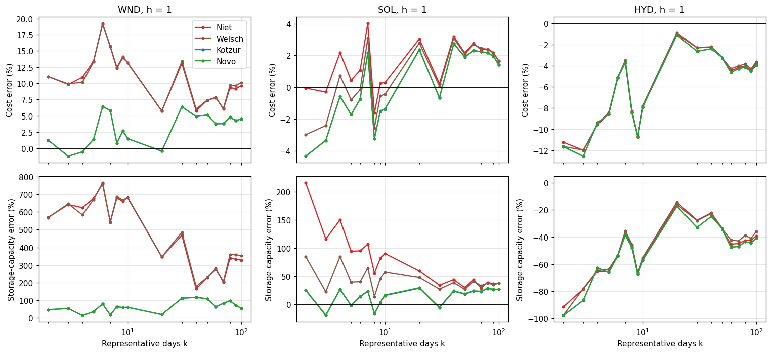
Errors are relative to the k365h1 Novo benchmark of the same resource and are computed from unrounded values.
[ ]:
res = results_source()
t4 = rp.table4(res)
display(t4.style.format({'Total cost': '{:,.0f}', 'Cost error (%)': '{:+.1f}', 'Storage capacity (kW·yr)': '{:.2f}',
                         'Capacity error (%)': '{:+.1f}', 'Runtime (s)': '{:.2f}', 'Memory (MB)': '{:.1f}'}))
| Scenario | Case | Formulation | Total cost | Cost error (%) | Storage capacity (kW·yr) | Capacity error (%) | Runtime (s) | Memory (MB) | |
|---|---|---|---|---|---|---|---|---|---|
| 0 | WND | k365h1 | Niet | 51,016 | -0.0 | 0.96 | -0.0 | 134.68 | 193.0 |
| 1 | WND | k365h1 | Welsch | 51,054 | +0.1 | 0.99 | +3.9 | 256.97 | 1051.7 |
| 2 | WND | k365h1 | Kotzur | 51,014 | -0.0 | 0.96 | -0.2 | 156.29 | 613.4 |
| 3 | WND | k365h1 | Novo | 51,016 | +0.0 | 0.96 | +0.0 | 427.28 | 10814.0 |
| 4 | WND | k8h1 | Niet | 57,305 | +12.3 | 7.45 | +678.9 | 0.30 | 4.9 |
| 5 | WND | k8h1 | Welsch | 57,380 | +12.5 | 7.53 | +686.7 | 0.67 | 13.9 |
| 6 | WND | k8h1 | Kotzur | 51,419 | +0.8 | 1.57 | +63.9 | 0.53 | 6.5 |
| 7 | WND | k8h1 | Novo | 51,424 | +0.8 | 1.57 | +64.4 | 6.17 | 281.7 |
| 8 | WND | k20h1 | Niet | 53,945 | +5.7 | 4.28 | +347.0 | 0.73 | 11.2 |
| 9 | WND | k20h1 | Welsch | 53,942 | +5.7 | 4.27 | +346.7 | 1.36 | 35.0 |
| 10 | WND | k20h1 | Kotzur | 50,811 | -0.4 | 1.14 | +19.5 | 0.67 | 13.2 |
| 11 | WND | k20h1 | Novo | 50,821 | -0.4 | 1.15 | +20.5 | 12.84 | 635.2 |
| 12 | SOL | k365h1 | Niet | 153,330 | -0.0 | 3.42 | -0.0 | 115.51 | 185.8 |
| 13 | SOL | k365h1 | Welsch | 153,353 | +0.0 | 3.44 | +0.7 | 242.08 | 1042.0 |
| 14 | SOL | k365h1 | Kotzur | 153,298 | -0.0 | 3.39 | -1.0 | 61.94 | 621.3 |
| 15 | SOL | k365h1 | Novo | 153,330 | +0.0 | 3.42 | +0.0 | 421.55 | 12195.1 |
| 16 | SOL | k9h1 | Niet | 153,697 | +0.2 | 6.21 | +81.6 | 0.31 | 5.2 |
| 17 | SOL | k9h1 | Welsch | 152,467 | -0.6 | 4.98 | +45.6 | 0.71 | 15.4 |
| 18 | SOL | k9h1 | Kotzur | 150,998 | -1.5 | 3.51 | +2.6 | 0.38 | 6.9 |
| 19 | SOL | k9h1 | Novo | 151,023 | -1.5 | 3.53 | +3.3 | 7.00 | 308.9 |
| 20 | SOL | k20h1 | Niet | 157,988 | +3.0 | 5.44 | +59.1 | 0.83 | 12.0 |
| 21 | SOL | k20h1 | Welsch | 157,591 | +2.8 | 5.04 | +47.5 | 3.28 | 34.5 |
| 22 | SOL | k20h1 | Kotzur | 156,927 | +2.3 | 4.38 | +28.1 | 1.03 | 13.9 |
| 23 | SOL | k20h1 | Novo | 156,960 | +2.4 | 4.41 | +29.1 | 13.30 | 634.9 |
| 24 | HYD | k365h1 | Niet | 90,841 | -0.0 | 6.06 | -0.0 | 319.63 | 193.0 |
| 25 | HYD | k365h1 | Welsch | 90,853 | +0.0 | 6.07 | +0.2 | 294.54 | 1051.7 |
| 26 | HYD | k365h1 | Kotzur | 90,836 | -0.0 | 6.06 | -0.1 | 82.98 | 613.4 |
| 27 | HYD | k365h1 | Novo | 90,841 | +0.0 | 6.06 | +0.0 | 491.14 | 10814.0 |
| 28 | HYD | k7h1 | Niet | 87,513 | -3.7 | 3.76 | -37.9 | 0.36 | 4.4 |
| 29 | HYD | k7h1 | Welsch | 87,659 | -3.5 | 3.91 | -35.5 | 0.56 | 12.2 |
| 30 | HYD | k7h1 | Kotzur | 87,473 | -3.7 | 3.72 | -38.6 | 0.32 | 6.0 |
| 31 | HYD | k7h1 | Novo | 87,473 | -3.7 | 3.72 | -38.6 | 5.25 | 252.3 |
| 32 | HYD | k20h1 | Niet | 89,921 | -1.0 | 5.09 | -16.0 | 1.03 | 11.2 |
| 33 | HYD | k20h1 | Welsch | 90,016 | -0.9 | 5.19 | -14.4 | 2.15 | 35.0 |
| 34 | HYD | k20h1 | Kotzur | 89,831 | -1.1 | 5.00 | -17.5 | 0.88 | 14.4 |
| 35 | HYD | k20h1 | Novo | 89,832 | -1.1 | 5.00 | -17.5 | 11.36 | 635.2 |
Traceability check. The Table 4 values of the paper are entered below and compared with the recomputed values. Costs and capacities agree exactly. Some capacity errors differ by up to ~3 percentage points because the paper divides by the benchmark rounded to two decimals (e.g. WND k8h1 Niet: 7.45/0.96 − 1 = +676.0 % versus +678.9 % unrounded).
[ ]:
draft = pd.DataFrame([  # Table 4 of the paper (cost error %, capacity error %)
 ('WND','k8h1','Niet',57305,12.3,7.45,676.0),('WND','k8h1','Welsch',57380,12.5,7.53,684.4),('WND','k8h1','Kotzur',51419,0.8,1.57,63.5),('WND','k8h1','Novo',51424,0.8,1.57,63.5),
 ('WND','k20h1','Niet',53945,5.7,4.28,345.8),('WND','k20h1','Welsch',53942,5.7,4.27,344.8),('WND','k20h1','Kotzur',50811,-0.4,1.14,18.7),('WND','k20h1','Novo',50821,-0.4,1.15,19.8),
 ('SOL','k9h1','Niet',153697,0.2,6.21,81.6),('SOL','k9h1','Welsch',152467,-0.6,4.98,45.6),('SOL','k9h1','Kotzur',150998,-1.5,3.51,2.6),('SOL','k9h1','Novo',151023,-1.5,3.53,3.2),
 ('SOL','k20h1','Niet',157988,3.0,5.44,59.1),('SOL','k20h1','Welsch',157591,2.8,5.04,47.4),('SOL','k20h1','Kotzur',156927,2.3,4.38,28.1),('SOL','k20h1','Novo',156960,2.4,4.41,28.9),
 ('HYD','k7h1','Niet',87513,-3.7,3.76,-38.0),('HYD','k7h1','Welsch',87659,-3.5,3.91,-35.5),('HYD','k7h1','Kotzur',87473,-3.7,3.72,-38.6),('HYD','k7h1','Novo',87473,-3.7,3.72,-38.6),
 ('HYD','k20h1','Niet',89921,-1.0,5.09,-16.0),('HYD','k20h1','Welsch',90016,-0.9,5.19,-14.4),('HYD','k20h1','Kotzur',89831,-1.1,5.00,-17.5),('HYD','k20h1','Novo',89832,-1.1,5.00,-17.5)],
 columns=['Scenario','Case','Formulation','cost_draft','cost_err_draft','cap_draft','cap_err_draft'])
tr = draft.merge(t4, on=['Scenario', 'Case', 'Formulation'])
tr['cost diff'] = tr['Total cost'].round(0) - tr['cost_draft']
tr['cap diff'] = tr['Storage capacity (kW·yr)'].round(2) - tr['cap_draft']
tr['cost-err diff (pp)'] = tr['Cost error (%)'].round(1) - tr['cost_err_draft']
tr['cap-err diff (pp)'] = tr['Capacity error (%)'].round(1) - tr['cap_err_draft']
display(tr[['Scenario', 'Case', 'Formulation', 'cost diff', 'cap diff', 'cost-err diff (pp)', 'cap-err diff (pp)']])
| Scenario | Case | Formulation | cost diff | cap diff | cost-err diff (pp) | cap-err diff (pp) | |
|---|---|---|---|---|---|---|---|
| 0 | WND | k8h1 | Niet | 0.0 | 0.0 | 0.0 | 2.9 |
| 1 | WND | k8h1 | Welsch | 0.0 | 0.0 | 0.0 | 2.3 |
| 2 | WND | k8h1 | Kotzur | 0.0 | 0.0 | 0.0 | 0.4 |
| 3 | WND | k8h1 | Novo | 0.0 | 0.0 | 0.0 | 0.9 |
| 4 | WND | k20h1 | Niet | 0.0 | 0.0 | 0.0 | 1.2 |
| 5 | WND | k20h1 | Welsch | 0.0 | 0.0 | 0.0 | 1.9 |
| 6 | WND | k20h1 | Kotzur | 0.0 | 0.0 | 0.0 | 0.8 |
| 7 | WND | k20h1 | Novo | 0.0 | 0.0 | 0.0 | 0.7 |
| 8 | SOL | k9h1 | Niet | 0.0 | 0.0 | 0.0 | 0.0 |
| 9 | SOL | k9h1 | Welsch | 0.0 | 0.0 | 0.0 | 0.0 |
| 10 | SOL | k9h1 | Kotzur | 0.0 | 0.0 | 0.0 | 0.0 |
| 11 | SOL | k9h1 | Novo | 0.0 | 0.0 | 0.0 | 0.1 |
| 12 | SOL | k20h1 | Niet | 0.0 | 0.0 | 0.0 | 0.0 |
| 13 | SOL | k20h1 | Welsch | 0.0 | 0.0 | 0.0 | 0.1 |
| 14 | SOL | k20h1 | Kotzur | 0.0 | 0.0 | 0.0 | 0.0 |
| 15 | SOL | k20h1 | Novo | 0.0 | 0.0 | 0.0 | 0.2 |
| 16 | HYD | k7h1 | Niet | 0.0 | 0.0 | 0.0 | 0.1 |
| 17 | HYD | k7h1 | Welsch | 0.0 | 0.0 | 0.0 | 0.0 |
| 18 | HYD | k7h1 | Kotzur | 0.0 | 0.0 | 0.0 | 0.0 |
| 19 | HYD | k7h1 | Novo | 0.0 | 0.0 | 0.0 | 0.0 |
| 20 | HYD | k20h1 | Niet | 0.0 | 0.0 | 0.0 | 0.0 |
| 21 | HYD | k20h1 | Welsch | 0.0 | 0.0 | 0.0 | 0.0 |
| 22 | HYD | k20h1 | Kotzur | 0.0 | 0.0 | 0.0 | 0.0 |
| 23 | HYD | k20h1 | Novo | 0.0 | 0.0 | 0.0 | 0.0 |
[ ]:
d = rp.add_errors(res[~res.limited])      # benchmark must be present when errors are computed
d = d[d.k != 365]
fig, axes = plt.subplots(2, 3, figsize=(14, 6.5), sharex=True)
for j, r in enumerate(['WND', 'SOL', 'HYD']):
    for f in ['Niet', 'Welsch', 'Kotzur', 'Novo']:
        g = d[(d.resource == r) & (d.formulation == f) & (d.h == 1)].sort_values('k')
        axes[0, j].plot(g.k, g.cost_err_pct, marker='o', ms=3, color=COLORS[f], label=f)
        axes[1, j].plot(g.k, g.cap_err_pct, marker='o', ms=3, color=COLORS[f], label=f)
    axes[0, j].set(title=f'{r}, h = 1', ylabel='Cost error (%)'); axes[1, j].set(xlabel='Representative days k', ylabel='Storage-capacity error (%)', xscale='log')
    for a in axes[:, j]: a.axhline(0, color='k', lw=.6)
axes[0, 0].legend(); plt.tight_layout(); plt.show()

# intra-day resolution: cost error vs h (median over k)
piv = d.groupby(['resource', 'formulation', 'h']).cost_err_pct.apply(lambda x: x.abs().median()).unstack('h')
display(piv.round(2).style.set_caption('Median |cost error| (%) across k, by block length h'))
| h | 1 | 2 | 4 | 6 | 8 | 12 | |
|---|---|---|---|---|---|---|---|
| resource | formulation | ||||||
| HYD | Kotzur | 4.600000 | 4.600000 | 4.620000 | 4.620000 | 4.630000 | 4.650000 |
| Niet | 4.470000 | 4.470000 | 4.480000 | 4.480000 | 4.490000 | 4.510000 | |
| Novo | 4.600000 | 4.600000 | 4.620000 | 4.620000 | 4.630000 | 4.650000 | |
| Welsch | 4.310000 | 4.320000 | 4.340000 | 4.360000 | 4.380000 | 4.430000 | |
| SOL | Kotzur | 2.050000 | 1.940000 | 1.670000 | 1.640000 | 1.650000 | 5.670000 |
| Niet | 1.900000 | 1.970000 | 1.580000 | 1.220000 | 1.110000 | 4.850000 | |
| Novo | 2.060000 | 1.940000 | 1.670000 | 1.640000 | 1.650000 | 5.670000 | |
| Welsch | 2.260000 | 2.130000 | 1.700000 | 1.400000 | 1.520000 | 4.820000 | |
| WND | Kotzur | 3.790000 | 3.760000 | 3.690000 | 3.640000 | 3.440000 | 3.110000 |
| Niet | 10.380000 | 10.280000 | 10.170000 | 10.210000 | 10.170000 | 9.790000 | |
| Novo | 3.800000 | 3.780000 | 3.710000 | 3.660000 | 3.460000 | 3.120000 | |
| Welsch | 10.130000 | 10.050000 | 9.920000 | 9.910000 | 9.880000 | 9.680000 |
[ ]:
# Computational burden (all aggregated configurations)
cb = res[~res.limited].groupby(['resource', 'formulation'])[['total_time_s', 'memory_MB']].median().unstack('formulation')
display(cb.round(2).style.set_caption('Median matrix-generation + solve time (s) and memory (MB)'))
| total_time_s | memory_MB | |||||||
|---|---|---|---|---|---|---|---|---|
| formulation | Kotzur | Niet | Novo | Welsch | Kotzur | Niet | Novo | Welsch |
| resource | ||||||||
| HYD | 0.280000 | 0.210000 | 0.940000 | 0.290000 | 6.000000 | 3.200000 | 43.100000 | 5.800000 |
| SOL | 0.330000 | 0.250000 | 1.040000 | 0.320000 | 5.900000 | 3.200000 | 43.000000 | 5.800000 |
| WND | 0.270000 | 0.210000 | 0.960000 | 0.250000 | 6.000000 | 3.200000 | 43.100000 | 5.800000 |
9. Binding storage-capacity stress test (Section 4.4; Figures 9–10)#
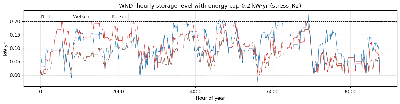
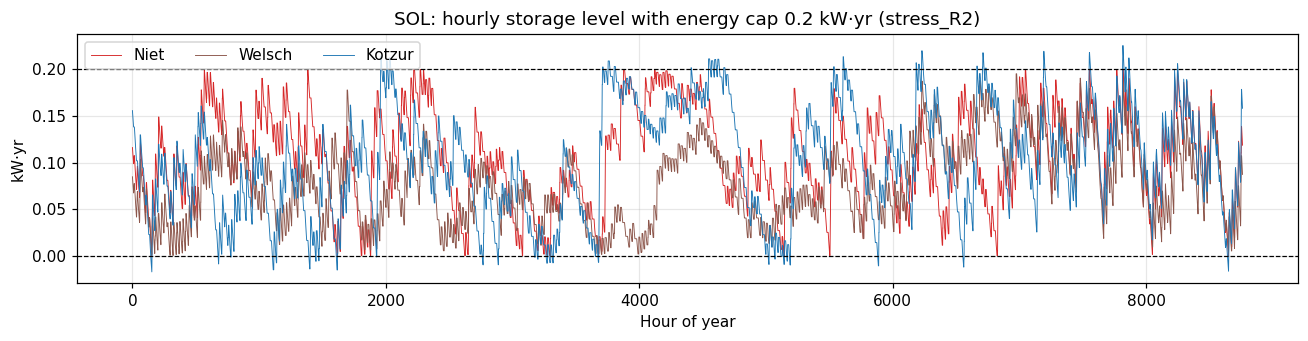
Full-year hourly runs with total storage energy capacity capped at 0.2 kW·yr (StorageMaxCapacity = 0.2; reported new capacity is then 0.15 because 0.05 is residual). Kotzur verifies SoC only at day boundaries, so its reconstructed hourly trajectory can leave the bounds.
Two counting conventions are reported. Strict counts physically infeasible states (SoC > 0.2 or < 0). At or beyond also counts hours exactly at the upper bound, which are feasible; the wind figure in the paper (224 h; 183 above) corresponds to this second convention.
[ ]:
if RUN_STRESS:
    for r in ['WND', 'SOL']:
        rp.run_case(r, 365, 1, cap=rp.STRESS_CAP, results_dir=FRESH, verbose=True)

STRESS_SOURCES = {'fresh': FRESH, 'regenerated (paper inputs)': PUBLISHED / 'stress_R2', 'archive': ARCH_LIM}
rows = []
for r in ['WND', 'SOL']:
    name = f'k365h1{r}_limited'
    for label, d_ in STRESS_SOURCES.items():
        if not (d_ / f'{name}_Storage_Level_Model_Kotzur_intraday.csv').exists():
            continue
        tab = rp.load_results(d_ / 'Simulation_Results.xlsx')   # cap is not encoded in file names
        t = tab[tab.Scenario == name].set_index('formulation')
        cap = t.loc['Kotzur', 'Storage Capacity'] + rp.RESIDUAL_STORAGE
        for f, m in [('Kotzur', 'Kotzur_intraday'), ('Niet', 'Niet'), ('Novo', 'Cluster'), ('Welsch', 'Welsch_intraday')]:
            if (d_ / f'{name}_Storage_Level_Model_{m}.csv').exists():
                v = rp.soc_violations(rp.read_storage(d_, name, m), upper=cap)
                rows.append({'resource': r, 'source': label, 'formulation': f, 'cap (kW.yr)': round(cap, 4),
                             'total cost': t.loc[f, 'Total cost'] if f in t.index else np.nan, **v})
stress = pd.DataFrame(rows)
display(stress.round(4))
| resource | source | formulation | cap (kW.yr) | total cost | n | max | min | above_strict | below_strict | total_strict | share_strict_pct | at_or_above_upper | total_if_counting_at_bound | share_if_counting_at_bound_pct | |
|---|---|---|---|---|---|---|---|---|---|---|---|---|---|---|---|
| 0 | WND | regenerated (paper inputs) | Kotzur | 0.2 | 136990.7749 | 8760 | 0.2274 | -0.0295 | 67 | 40 | 107 | 1.2215 | 187 | 227 | 2.5913 |
| 1 | WND | regenerated (paper inputs) | Niet | 0.2 | 227531.9429 | 8760 | 0.2000 | 0.0000 | 0 | 0 | 0 | 0.0000 | 197 | 197 | 2.2489 |
| 2 | WND | regenerated (paper inputs) | Welsch | 0.2 | 227533.1312 | 8760 | 0.2000 | 0.0000 | 0 | 0 | 0 | 0.0000 | 1 | 1 | 0.0114 |
| 3 | WND | archive | Kotzur | 0.2 | 126111.2565 | 8760 | 0.2213 | -0.0271 | 114 | 41 | 155 | 1.7694 | 183 | 224 | 2.5571 |
| 4 | WND | archive | Niet | 0.2 | 136451.2731 | 8760 | 0.2000 | 0.0000 | 0 | 0 | 0 | 0.0000 | 13 | 13 | 0.1484 |
| 5 | WND | archive | Novo | 0.2 | 136451.4557 | 8760 | 0.2000 | 0.0000 | 0 | 0 | 0 | 0.0000 | 60 | 60 | 0.6849 |
| 6 | WND | archive | Welsch | 0.2 | 143270.6770 | 8760 | 0.1956 | -0.0000 | 0 | 0 | 0 | 0.0000 | 0 | 0 | 0.0000 |
| 7 | SOL | regenerated (paper inputs) | Kotzur | 0.2 | 413582.2431 | 8760 | 0.2258 | -0.0175 | 267 | 215 | 482 | 5.5023 | 277 | 492 | 5.6164 |
| 8 | SOL | regenerated (paper inputs) | Niet | 0.2 | 426705.3476 | 8760 | 0.2000 | 0.0000 | 0 | 0 | 0 | 0.0000 | 45 | 45 | 0.5137 |
| 9 | SOL | regenerated (paper inputs) | Welsch | 0.2 | 457891.1365 | 8760 | 0.1954 | 0.0000 | 0 | 0 | 0 | 0.0000 | 0 | 0 | 0.0000 |
| 10 | SOL | archive | Kotzur | 3.0 | 168474.9062 | 8760 | 3.0186 | -0.0147 | 11 | 25 | 36 | 0.4110 | 12 | 37 | 0.4224 |
| 11 | SOL | archive | Niet | 3.0 | 169694.4204 | 8760 | 3.0000 | 0.0000 | 0 | 0 | 0 | 0.0000 | 2 | 2 | 0.0228 |
| 12 | SOL | archive | Novo | 3.0 | 169694.6618 | 8760 | 3.0000 | 0.0000 | 0 | 0 | 0 | 0.0000 | 1 | 1 | 0.0114 |
| 13 | SOL | archive | Welsch | 3.0 | 170590.3639 | 8760 | 2.9853 | 0.0000 | 0 | 0 | 0 | 0.0000 | 0 | 0 | 0.0000 |
Provenance of the Section 4.4 numbers.
Solar: the regenerated run with the paper’s inputs reproduces the values in the paper exactly (max 0.2258, min −0.0175, 267 h above, 215 h below, 482 h = 5.50 %, strict counting). The archived solar “limited” run used a cap of 3.0 kW·yr and is unrelated.
Wind: the values in the paper (max 0.2213, min −0.0271) come from the archived run, whose costs differ from a run with the paper’s inputs, so that run used different inputs from the main study. The regenerated wind run uses the paper’s inputs. Counted strictly, like solar, its hours above the bound exclude hours exactly at the bound; the figure of 183 h in the paper includes them.
The regenerated runs omit Novo, which needs ~12 GB of RAM at k365h1; Novo does not affect the Kotzur trajectory. Set
RUN_STRESS = Trueon a 16 GB machine to complete them.Cost column: under the binding cap, Kotzur’s total cost is clearly lower than that of the formulations that keep SoC within bounds. The violations therefore do change total cost.
[ ]:
for r in ['WND', 'SOL']:
    name = f'k365h1{r}_limited'
    d_ = next((d for d in STRESS_SOURCES.values() if (d / f'{name}_Storage_Level_Model_Kotzur_intraday.csv').exists()), None)
    if d_ is None:
        continue
    cap = stress[(stress.resource == r) & (stress.source == [k for k, v in STRESS_SOURCES.items() if v == d_][0])]['cap (kW.yr)'].iloc[0]
    fig, ax = plt.subplots(figsize=(12, 3.2))
    for f, m in [('Niet', 'Niet'), ('Novo', 'Cluster'), ('Welsch', 'Welsch_intraday'), ('Kotzur', 'Kotzur_intraday')]:
        p = d_ / f'{name}_Storage_Level_Model_{m}.csv'
        if p.exists():
            ax.plot(rp.read_storage(d_, name, m), lw=.6, color=COLORS[f], label=f)
    ax.axhline(cap, color='k', ls='--', lw=.8); ax.axhline(0, color='k', ls='--', lw=.8)
    ax.set(title=f'{r}: hourly storage level with energy cap {cap} kW·yr ({d_.name})', xlabel='Hour of year', ylabel='kW·yr')
    ax.legend(ncol=4); plt.tight_layout(); plt.show()
10. SoC fidelity metrics (Section 4.3; Figure 8)#
The repository did not contain the script used for Figure 8, so the metrics are re-implemented here with explicit definitions:
each aggregated trajectory is expanded to 8760 h (Novo and Kotzur: chronological blocks, Kotzur reconstructed; Welsch: its reconstructed trajectory in native grouped day-type order, as in
graph_generator.py; Niet: representative blocks held for their year-split duration);MAE, RMSE and Pearson r against the k365h1 benchmark;
rainflow counting (ASTM E1049, half cycles = 0.5) of each trajectory, compared with the benchmark count.
Values may differ from the published Figure 8 if the original script used other alignment conventions; the definitions above are the ones used here.
[ ]:
CASES = [('WND', 8, 1), ('WND', 20, 1), ('SOL', 9, 1), ('SOL', 20, 1), ('HYD', 7, 1), ('HYD', 20, 1)]
rows = []
for r, k, h in CASES:
    name = f'k{k}h{h}{r}'
    d_ = FRESH if (FRESH / f'{name}_Storage_Level_Model_Cluster.csv').exists() else ARCH_MAIN
    bdir = FRESH if (FRESH / f'k365h1{r}_Storage_Level_Model_Niet.csv').exists() else ARCH_MAIN
    if not (d_ / f'{name}_Storage_Level_Model_Cluster.csv').exists():
        print(f'{name}: trajectories not available (download the full archive)'); continue
    b = rp.read_storage(bdir, f'k365h1{r}', 'Niet').to_numpy()
    for f in ['Niet', 'Welsch', 'Kotzur', 'Novo']:
        try:
            t = rp.hourly_trajectory(d_, name, f, h)
            rows.append({'case': name, 'formulation': f, **rp.fidelity_metrics(b, t)})
        except FileNotFoundError as e:
            print(e)
fid = pd.DataFrame(rows)
if fid.empty:
    print('No trajectories found: place the full archive in data/full_archive/ or run the cases.')
else:
    fid['cycle error (%)'] = 100 * (fid.rainflow_cycles / fid.rainflow_cycles_benchmark - 1)
    display(fid.round(4))
| case | formulation | MAE | RMSE | Pearson | rainflow_cycles | rainflow_cycles_benchmark | cycle error (%) | |
|---|---|---|---|---|---|---|---|---|
| 0 | k8h1WND | Niet | 3.8406 | 4.5450 | -0.7621 | 6.0 | 241.5 | -97.5155 |
| 1 | k8h1WND | Welsch | 3.9106 | 4.6406 | -0.7562 | 199.0 | 241.5 | -17.5983 |
| 2 | k8h1WND | Kotzur | 0.3393 | 0.3993 | 0.9178 | 187.5 | 241.5 | -22.3602 |
| 3 | k8h1WND | Novo | 0.3432 | 0.4030 | 0.9178 | 187.5 | 241.5 | -22.3602 |
| 4 | k20h1WND | Niet | 1.5785 | 1.8523 | -0.2928 | 16.0 | 241.5 | -93.3747 |
| 5 | k20h1WND | Welsch | 1.5190 | 1.7895 | -0.2894 | 210.0 | 241.5 | -13.0435 |
| 6 | k20h1WND | Kotzur | 0.1517 | 0.1914 | 0.8344 | 189.0 | 241.5 | -21.7391 |
| 7 | k20h1WND | Novo | 0.1535 | 0.1938 | 0.8344 | 189.0 | 241.5 | -21.7391 |
| 8 | k9h1SOL | Niet | 1.2404 | 1.4084 | 0.8868 | 8.5 | 354.5 | -97.6023 |
| 9 | k9h1SOL | Welsch | 0.6273 | 0.7672 | 0.9487 | 323.5 | 354.5 | -8.7447 |
| 10 | k9h1SOL | Kotzur | 0.1277 | 0.1673 | 0.9913 | 323.5 | 354.5 | -8.7447 |
| 11 | k9h1SOL | Novo | 0.1289 | 0.1690 | 0.9913 | 323.5 | 354.5 | -8.7447 |
| 12 | k20h1SOL | Niet | 1.0992 | 1.3273 | 0.7925 | 18.5 | 354.5 | -94.7814 |
| 13 | k20h1SOL | Welsch | 0.9626 | 1.1868 | 0.8120 | 346.5 | 354.5 | -2.2567 |
| 14 | k20h1SOL | Kotzur | 0.4245 | 0.5515 | 0.9899 | 346.5 | 354.5 | -2.2567 |
| 15 | k20h1SOL | Novo | 0.4332 | 0.5625 | 0.9899 | 346.5 | 354.5 | -2.2567 |
| 16 | k7h1HYD | Niet | 1.9531 | 2.5262 | 0.4167 | 5.5 | 43.5 | -87.3563 |
| 17 | k7h1HYD | Welsch | 1.9295 | 2.4960 | 0.4201 | 240.5 | 43.5 | 452.8736 |
| 18 | k7h1HYD | Kotzur | 1.9228 | 2.3137 | 0.7956 | 264.0 | 43.5 | 506.8966 |
| 19 | k7h1HYD | Novo | 1.9228 | 2.3137 | 0.7956 | 264.0 | 43.5 | 506.8966 |
| 20 | k20h1HYD | Niet | 1.2624 | 1.4574 | 0.8011 | 15.0 | 43.5 | -65.5172 |
| 21 | k20h1HYD | Welsch | 1.2380 | 1.4223 | 0.7972 | 255.0 | 43.5 | 486.2069 |
| 22 | k20h1HYD | Kotzur | 1.0184 | 1.2421 | 0.9344 | 287.0 | 43.5 | 559.7701 |
| 23 | k20h1HYD | Novo | 1.0184 | 1.2421 | 0.9344 | 287.0 | 43.5 | 559.7701 |
11. Seed sensitivity of system cost#
Re-solves selected configurations with seeds 1 and 2 and compares total-cost error with seed 0. The question is whether the seed-induced spread is small compared with the differences between formulations.
[ ]:
SEED_DIR = REPO / 'results' / 'seeds'
if RUN_SEED_COSTS:
    for s in [1, 2]:
        for r in ['WND', 'SOL', 'HYD']:
            for k in [4, 8, 20]:
                rp.run_case(r, k, 1, random_state=s, results_dir=SEED_DIR, suffix=f'_s{s}', verbose=True)
sd = None
if (SEED_DIR / 'Simulation_Results.xlsx').exists():
    sd = rp.load_results(SEED_DIR / 'Simulation_Results.xlsx')
elif (PUBLISHED / 'seeds' / 'seed_runs.xlsx').exists():
    sd = rp.load_results(PUBLISHED / 'seeds' / 'seed_runs.xlsx')
if sd is not None:
    sd['seed'] = sd.Scenario.str.extract(r'_s(\d+)$')[0].astype(int)
    sd['resource'] = sd.Scenario.str.extract(r'(WND|SOL|HYD)')[0]
    _r = results_source()
    base = _r[(_r.h == 1) & _r.k.isin(sd.k.unique()) & ~_r.limited].assign(seed=0)
    allseeds = pd.concat([base, sd], ignore_index=True)
    bm = archive[(archive.k == 365) & (archive.Model == 'Model_Cluster')].set_index('resource')['Total cost']
    allseeds['cost_err_pct'] = 100 * (allseeds['Total cost'] / allseeds.resource.map(bm) - 1)
    piv = allseeds.pivot_table(index=['resource', 'k', 'formulation'], columns='seed', values='cost_err_pct')
    piv['seed spread (pp)'] = piv.max(1) - piv.min(1)
    display(piv.round(2))
    between = allseeds[allseeds.seed == 0].groupby(['resource', 'k']).cost_err_pct.agg(lambda x: x.max() - x.min())
    within = piv['seed spread (pp)'].groupby(level=[0, 1]).max()
    cmp_ = pd.DataFrame({'max seed spread (pp)': within, 'between-formulation range, seed 0 (pp)': between})
    display(cmp_.round(2))
    best = (allseeds.assign(a=allseeds.cost_err_pct.abs()).sort_values('a')
                    .groupby(['resource', 'k', 'seed']).formulation.first().unstack('seed'))
    display(best.rename_axis(columns='seed').style.set_caption('Formulation with the smallest |cost error|'))
    cap_piv = allseeds.pivot_table(index=['resource', 'k', 'formulation'], columns='seed',
                                   values='Storage Capacity')
    display(cap_piv.round(3).style.set_caption('Storage capacity (kW·yr) by seed'))
| seed | 0 | 1 | 2 | seed spread (pp) | ||
|---|---|---|---|---|---|---|
| resource | k | formulation | ||||
| HYD | 4 | Kotzur | -9.40 | -4.06 | -5.69 | 5.34 |
| Niet | -9.57 | -3.97 | -5.21 | 5.60 | ||
| Novo | -9.40 | -4.06 | -5.69 | 5.34 | ||
| Welsch | -9.53 | -3.90 | -5.29 | 5.63 | ||
| 8 | Kotzur | -8.46 | -7.16 | -3.31 | 5.15 | |
| Niet | -8.39 | -7.01 | -3.01 | 5.37 | ||
| Novo | -8.46 | -7.16 | -3.31 | 5.15 | ||
| Welsch | -8.31 | -6.95 | -3.03 | 5.28 | ||
| 20 | Kotzur | -1.11 | -4.91 | -5.94 | 4.82 | |
| Niet | -1.01 | -4.82 | -5.99 | 4.97 | ||
| Novo | -1.11 | -4.91 | -5.94 | 4.82 | ||
| Welsch | -0.91 | -4.80 | -5.90 | 4.99 | ||
| SOL | 4 | Kotzur | -0.59 | -0.40 | -1.58 | 1.17 |
| Niet | 2.18 | 2.40 | 1.29 | 1.11 | ||
| Novo | -0.57 | -0.39 | -1.56 | 1.17 | ||
| Welsch | 0.73 | 0.98 | -0.32 | 1.30 | ||
| 8 | Kotzur | -3.25 | -0.05 | -4.35 | 4.29 | |
| Niet | -1.63 | 1.72 | -2.48 | 4.20 | ||
| Novo | -3.23 | -0.04 | -4.32 | 4.29 | ||
| Welsch | -2.56 | 0.77 | -3.28 | 4.04 | ||
| 20 | Kotzur | 2.35 | 3.70 | -0.30 | 4.00 | |
| Niet | 3.04 | 4.67 | 0.84 | 3.83 | ||
| Novo | 2.37 | 3.71 | -0.29 | 4.00 | ||
| Welsch | 2.78 | 4.39 | 0.58 | 3.81 | ||
| WND | 4 | Kotzur | -0.50 | 0.33 | -0.77 | 1.10 |
| Niet | 10.93 | 11.67 | 10.81 | 0.86 | ||
| Novo | -0.50 | 0.33 | -0.77 | 1.10 | ||
| Welsch | 10.17 | 11.09 | 10.09 | 1.00 | ||
| 8 | Kotzur | 0.79 | 2.97 | 4.39 | 3.60 | |
| Niet | 12.33 | 10.86 | 14.20 | 3.34 | ||
| Novo | 0.80 | 2.99 | 4.41 | 3.61 | ||
| Welsch | 12.47 | 10.91 | 14.35 | 3.44 | ||
| 20 | Kotzur | -0.40 | 4.33 | 5.29 | 5.69 | |
| Niet | 5.74 | 9.38 | 13.75 | 8.01 | ||
| Novo | -0.38 | 4.34 | 5.30 | 5.69 | ||
| Welsch | 5.74 | 9.34 | 13.79 | 8.05 |
| max seed spread (pp) | between-formulation range, seed 0 (pp) | ||
|---|---|---|---|
| resource | k | ||
| HYD | 4 | 5.63 | 0.17 |
| 8 | 5.37 | 0.15 | |
| 20 | 4.99 | 0.20 | |
| SOL | 4 | 1.30 | 2.76 |
| 8 | 4.29 | 1.62 | |
| 20 | 4.00 | 0.69 | |
| WND | 4 | 1.10 | 11.43 |
| 8 | 3.61 | 11.68 | |
| 20 | 8.05 | 6.14 |
| seed | 0 | 1 | 2 | |
|---|---|---|---|---|
| resource | k | |||
| HYD | 4 | Novo | Welsch | Niet |
| 8 | Welsch | Welsch | Niet | |
| 20 | Welsch | Welsch | Welsch | |
| SOL | 4 | Novo | Novo | Welsch |
| 8 | Niet | Novo | Niet | |
| 20 | Kotzur | Kotzur | Novo | |
| WND | 4 | Novo | Kotzur | Novo |
| 8 | Kotzur | Kotzur | Kotzur | |
| 20 | Novo | Kotzur | Kotzur |
| seed | 0 | 1 | 2 | ||
|---|---|---|---|---|---|
| resource | k | formulation | |||
| HYD | 4 | Kotzur | 2.260000 | 3.115000 | 2.011000 |
| Niet | 2.106000 | 3.201000 | 2.448000 | ||
| Novo | 2.260000 | 3.115000 | 2.012000 | ||
| Welsch | 2.144000 | 3.263000 | 2.374000 | ||
| 8 | Kotzur | 3.171000 | 2.754000 | 3.915000 | |
| Niet | 3.238000 | 2.889000 | 4.184000 | ||
| Novo | 3.174000 | 2.754000 | 3.916000 | ||
| Welsch | 3.307000 | 2.941000 | 4.166000 | ||
| 20 | Kotzur | 5.002000 | 3.682000 | 3.967000 | |
| Niet | 5.091000 | 3.771000 | 3.921000 | ||
| Novo | 5.002000 | 3.682000 | 3.967000 | ||
| Welsch | 5.186000 | 3.788000 | 4.003000 | ||
| SOL | 4 | Kotzur | 4.303000 | 4.640000 | 3.395000 |
| Niet | 8.540000 | 8.938000 | 7.785000 | ||
| Novo | 4.324000 | 4.661000 | 3.417000 | ||
| Welsch | 6.320000 | 6.761000 | 5.325000 | ||
| 8 | Kotzur | 2.830000 | 3.146000 | 3.915000 | |
| Niet | 5.312000 | 5.871000 | 6.780000 | ||
| Novo | 2.851000 | 3.169000 | 3.946000 | ||
| Welsch | 3.878000 | 4.402000 | 5.550000 | ||
| 20 | Kotzur | 4.379000 | 4.806000 | 3.752000 | |
| Niet | 5.441000 | 6.291000 | 5.505000 | ||
| Novo | 4.413000 | 4.823000 | 3.768000 | ||
| Welsch | 5.043000 | 5.864000 | 5.104000 | ||
| WND | 4 | Kotzur | 1.094000 | 1.130000 | 1.121000 |
| Niet | 6.926000 | 6.915000 | 7.028000 | ||
| Novo | 1.094000 | 1.130000 | 1.121000 | ||
| Welsch | 6.535000 | 6.618000 | 6.663000 | ||
| 8 | Kotzur | 1.569000 | 1.197000 | 2.230000 | |
| Niet | 7.454000 | 5.223000 | 7.233000 | ||
| Novo | 1.573000 | 1.209000 | 2.235000 | ||
| Welsch | 7.529000 | 5.246000 | 7.309000 | ||
| 20 | Kotzur | 1.144000 | 1.557000 | 2.173000 | |
| Niet | 4.277000 | 4.134000 | 6.490000 | ||
| Novo | 1.153000 | 1.564000 | 2.181000 | ||
| Welsch | 4.274000 | 4.113000 | 6.509000 |
Reading the result. Seed-induced spreads in cost error reach several percentage points (largest for HYD and WND at k = 20). For HYD the spread exceeds the between-formulation differences, while for WND at small k the gap between {Kotzur, Novo} and {Niet, Welsch} remains larger than the seed spread (WND k ≤ 8: separation 7.9–11.5 pp vs spread ≤ 3.6 pp). The qualitative grouping of formulations is therefore robust, but individual error levels in Table 4 depend on the clustering.
11.1 Why the wind gap between formulations narrows with k#
In Niet (constraint S2, Eq. 1) each representative hour’s net storage flow is multiplied by YearSplit, so one hour of a representative day lasts N_c hours, N_c being the number of days in its cluster. The representative days are chained in date order of the medoid days (cluster.py sorts them), not in the actual order of the 365 days. A cluster’s net imbalance therefore builds up without the reversals that the real day sequence would bring, and Niet sizes storage for swings that never
occur. Kotzur and Novo follow the actual day sequence. As k grows, N_c ≈ 365/k shrinks and so does this artificial swing. Welsch (one season) repeats each day type N_c days in a row instead; for wind the two readings give almost the same swing, for solar they do not.
rp.phantom_swing measures, without solving, how much swing Niet’s chaining adds over the actual order. The clean test is against Niet’s storage capacity error, because the cost gap mixes this effect with a second one: Kotzur and Novo also get worse at large k (with seed 0, cost error within ±3 % for k ≤ 20 except k = 6–7, and 4–6 % for every k ≥ 30), which the phantom swing does not explain.
[ ]:
bm = archive[(archive.k == 365) & (archive.Model == 'Model_Cluster')].set_index('resource')
wnd = archive[(archive.resource == 'WND') & (archive.h == 1) & (archive.k < 365) & ~archive.limited].copy()
wnd['cost_err_pct'] = 100 * (wnd['Total cost'] / bm.loc['WND', 'Total cost'] - 1)
wnd['stor_err_pct'] = 100 * (wnd['Storage Capacity'] / bm.loc['WND', 'Storage Capacity'] - 1)

mech = pd.DataFrame([rp.phantom_swing('WND', k) for k in rp.K_VALUES]).set_index('k')
for f in ['Niet', 'Kotzur']:
    m = wnd[wnd.formulation == f].set_index('k')
    mech[f'{f} storage err (%)'], mech[f'{f} cost err (%)'] = m.stor_err_pct, m.cost_err_pct
display(mech[['phantom_swing', 'phantom_swing_day_blocks', 'Niet storage err (%)', 'Niet cost err (%)',
              'Kotzur storage err (%)', 'Kotzur cost err (%)']].round(3).T)
r = lambda a, b, how='pearson': mech[a].corr(mech[b], method=how)
print('Seed 0, 18 values of k: phantom swing vs Niet storage error r = %.2f (rho = %.2f); vs Niet cost error r = %.2f'
      % (r('phantom_swing', 'Niet storage err (%)'), r('phantom_swing', 'Niet storage err (%)', 'spearman'),
         r('phantom_swing', 'Niet cost err (%)')))

fig, axs = plt.subplots(1, 2, figsize=(11, 4))
ax = axs[0]
sc = ax.scatter(mech.phantom_swing, mech['Niet storage err (%)'], c=np.log10(mech.index), cmap='viridis', s=28, zorder=3)
for k in [2, 4, 8, 20, 50, 100]:
    ax.annotate(f'k={k}', (mech.phantom_swing[k], mech['Niet storage err (%)'][k]), textcoords='offset points', xytext=(4, 3), fontsize=7)
if 'allseeds' in globals():   # seed runs from step 11
    sn = allseeds[(allseeds.resource == 'WND') & (allseeds.formulation == 'Niet')].copy()
    sn['stor_err_pct'] = 100 * (sn['Storage Capacity'] / bm.loc['WND', 'Storage Capacity'] - 1)
    sn['phantom_swing'] = [rp.phantom_swing('WND', k, s)['phantom_swing'] for k, s in zip(sn.k, sn.seed)]
    ax.scatter(sn.phantom_swing, sn.stor_err_pct, facecolors='none', edgecolors='k', s=40, label='seeds 0–2 (k = 4, 8, 20)')
    ax.legend(fontsize=8, loc='lower right')
    display(sn[['k', 'seed', 'phantom_swing', 'stor_err_pct']].sort_values(['k', 'seed']).round(3))
    print('Seed runs (WND, k = 4, 8, 20): phantom swing vs Niet storage error r = %.2f' % sn.phantom_swing.corr(sn.stor_err_pct))
ax.set(xlabel='Phantom storage swing (energy units)', ylabel='Niet storage capacity error (%)', title='(a) Niet, WND, h = 1')
fig.colorbar(sc, ax=ax, label='log$_{10}$ k')

ax = axs[1]   # the second effect: Kotzur/Novo drift at large k
for f in ['Niet', 'Welsch', 'Kotzur', 'Novo']:
    m = wnd[wnd.formulation == f].sort_values('k')
    ax.plot(range(len(m)), m.cost_err_pct, '--' if f == 'Novo' else '-', marker='o', ms=3, lw=1.2, color=COLORS[f], label=f)
ax.set_xticks(range(len(rp.K_VALUES)), labels=rp.K_VALUES, fontsize=7)
ax.axhline(0, color='0.5', lw=.8)
ax.set(xlabel='Representative days k', ylabel='Cost error (%)', title='(b) Cost error, WND, h = 1, seed 0')
ax.legend(frameon=False, fontsize=8)
plt.tight_layout(); plt.show()
Reading the result. The phantom swing tracks Niet’s storage capacity error (archived runs: r ≈ 0.87 across the 18 values of k, ≈ 0.90 across the nine seed runs), including the seed spread at k = 20: seed 2 gives both the largest swing and the largest storage error. It tracks Niet’s cost error less well (r ≈ 0.61), and it explains only Niet’s side of the narrowing. The other side is Kotzur and Novo getting worse for k ≥ 30 (panel b): their storage capacity rises to 1.5–2.1 kW·yr against 0.96 in the benchmark, although the input-level measures move the other way (their chronological swing and the represented annual energy are closest to the benchmark at large k). This effect is not explained here. Part of it is shared: the spikes at k = 6, 7 and 30 appear in all four formulations, so they come from the clustering, not from the storage formulation. Kotzur’s cost accuracy at small k is also partly cancellation: at k = 8 its cost error is +0.8 % but its storage error is +64 %.
What the results support: Niet and Welsch cost more than Kotzur and Novo for all 18 values of k with seed 0 and in all nine seed runs. Seed sensitivity was measured only at k = 4, 8 and 20; at k = 20 the gap (5.0–8.5 pp) is comparable to the seed-induced spread (up to 8.1 pp).
12. Where each published number comes from#
Claim in the paper |
Reproduced in |
|---|---|
Section 3.2 clustering settings |
Step 3 |
Section 4.1 hand-calculated SoC check |
Step 4 ( |
Figure 6, Table S1 |
Step 6 |
Table 4, Figure 7, Tables S2–S4 |
Steps 7–8 |
Section 4.4 wind/solar violation statistics, Figures 9–10 |
Step 9 |
Figure 8 metrics |
Step 10 (re-implementation) |
C2 multi-seed robustness |
Steps 3.1 and 11 |
Fresh runs go to results/; the archive is in data/published_results/ (tables and key trajectories) and, in full, in the Zenodo record cited in the Data Availability Statement.