RESource Builder Module#
Quick Start with run.py#
The enhanced run.py script provides the simplest way to execute complete resource assessments with flexible region selection and colored output.
Command Overview#
Usage Pattern |
Example |
Description |
|---|---|---|
All Regions |
|
Process all regions in config |
Specific Regions |
|
Process selected regions only |
Default Config |
|
Use default Canadian config |
Validation |
|
Shows available regions |
Regional Support#
Region Set |
Config File |
Available Regions |
|---|---|---|
Canadian Provinces |
|
BC, QC, AB, SK, ON, NS, MB |
Western Balkans |
|
AL, BA, XK, ME, MK, RS |
Custom Regions |
User-defined config |
Defined in |
Advanced Usage: Step-by-Step Workflow#
Warning
Typical Sequential Steps involves the following process as mentioned below. Note that data-source errors, configuration error may break the workflow which may necessitate additional methods to be used as intermediate steps.
Tip
Check the open-access publication on RESource
See also
For detailed API documentation of the methods, see RES API References and apis under RESource Builder.
Step 1: Prepare Spatial Grid Cells#
See also
get_grid_cells() at RESource Builder of RES API References.
This method collects the sub-national administrative boundaries.
Using that boundary, we calculate the Minimum Bounding Rectangle (MBR).
We use that MBR as a cutout to source weather resources data from ERA5 via CDSAPI. The ERA5's cutout is then stored as a netcdf `.nc' file.
We load that cutout as
atlite'scutoutobject.We then use
atlite'scutout.gridattribute to create our test beds for the analysis i.e. the grid cells (geodataframe)We get the following key visuals out of this step:
Land availability map at excluder's highest resolution and another one at ERA5's resolution.
To harmonize the grid cells with the weather resources data, we use the ERA5's resolution data for further stages
Important
Data supply-chain for this method Requires CDS-API setup
The resulting GeoDataFrame from get_grid_cells() includes the following columns:
Attribute |
Description |
|---|---|
|
Longitude coordinate (center) of the grid cell |
|
Latitude coordinate (center) of the grid cell |
|
Name of the country containing the grid cell. This is datafield 'NAME_0' in GADM's dataset |
|
Name of the province or state containing the grid cell. This is datafield 'NAME_1' in GADM's dataset |
|
Name of the specific region containing the grid cell. This is datafield 'NAME_2' in GADM's dataset |
|
Polygon geometry defining the spatial extent of the grid cell. The default CRS is EPSG:4326, to be set via config file |
Step 2: Calculate Potential Capacity#
See also
RES.cell_processor.get_capacity() of RES API References.
This method loads the cutout (atlite's cutout object), regional boundary (GeoDataFrame), loads the cost parameters and also initiates a composite excluder
The (
atlite's exclusion container) to merge all the spatial layers.
the
cutout.availabilitymatrixmethod calculates % of usable area within each grid cell after applying exclusion criteria (e.g., protected areas, water bodies) and returns anAvaliabilityMatrixWe apply technology landuse intensity (e.g., MW/km² for wind or solar) to translate this to potential capacity data.
Attention
Current results gives a percentage of availability for each grid cell. It does not tell specifically which spatial area inside a grid cell is unavailable.
The potential capacity translation processing involves
areacalculation. The area calculation method is integrated toRES.cell_processor.get_capacity(). That method is sensitive to area calculation specific coordinate-system projection of the geodataframe. It is recommended to be cautious about choosing this crs.
We get the maximum installable capacity for each grid cell based on available area, land use constraints, and technology-specific parameters.
This method returns a named tuple with 'data' (a GeoDataFrame) and 'matrix' (availability matrix xarray).
Tip
You can access the individual elements of the named tuple using dot notation, e.g., it you named the methods results as
resultthenresult.data,result.matrix
Resulting GeoDataFrame includes the following new fields for each resource type (e.g., wind, solar):
Attribute |
Description |
|---|---|
|
Maximum installable capacity (MW) for the resource in the grid cell |
|
Capital expenditure per MW for the resource |
|
Fixed operation & maintenance cost per MW |
|
Variable operation & maintenance cost per MWh |
|
Estimated grid connection cost per km for the resource |
|
Transmission line rebuild cost per km for the resource |
|
Expected operational lifetime (years) for the resource |
Hint
Working enhancement includes VRE farm layout calculation models to make the potential capacity calculation more closer to the real world scenarios.
Future improvements are planned to identify spatial areas (geometry) inside a grid cell.
Step 3: Get CF and Windspeed from Higher Resolution Data#
Attention
Currently configured for Wind Resources only.
Why wind resources' ERA5 data are rescaled ? Wind resources (windspeed) are known to have significant variations across ERA5's ~30km resolution. To account for this, we rescaled the windspeed using higher resolution data from the Global Wind Atlas (GWA). This allows us to better estimate the windspeed at the grid cell level. However, GWA does not provide hourly profiles, so we source the profile from ERA5.
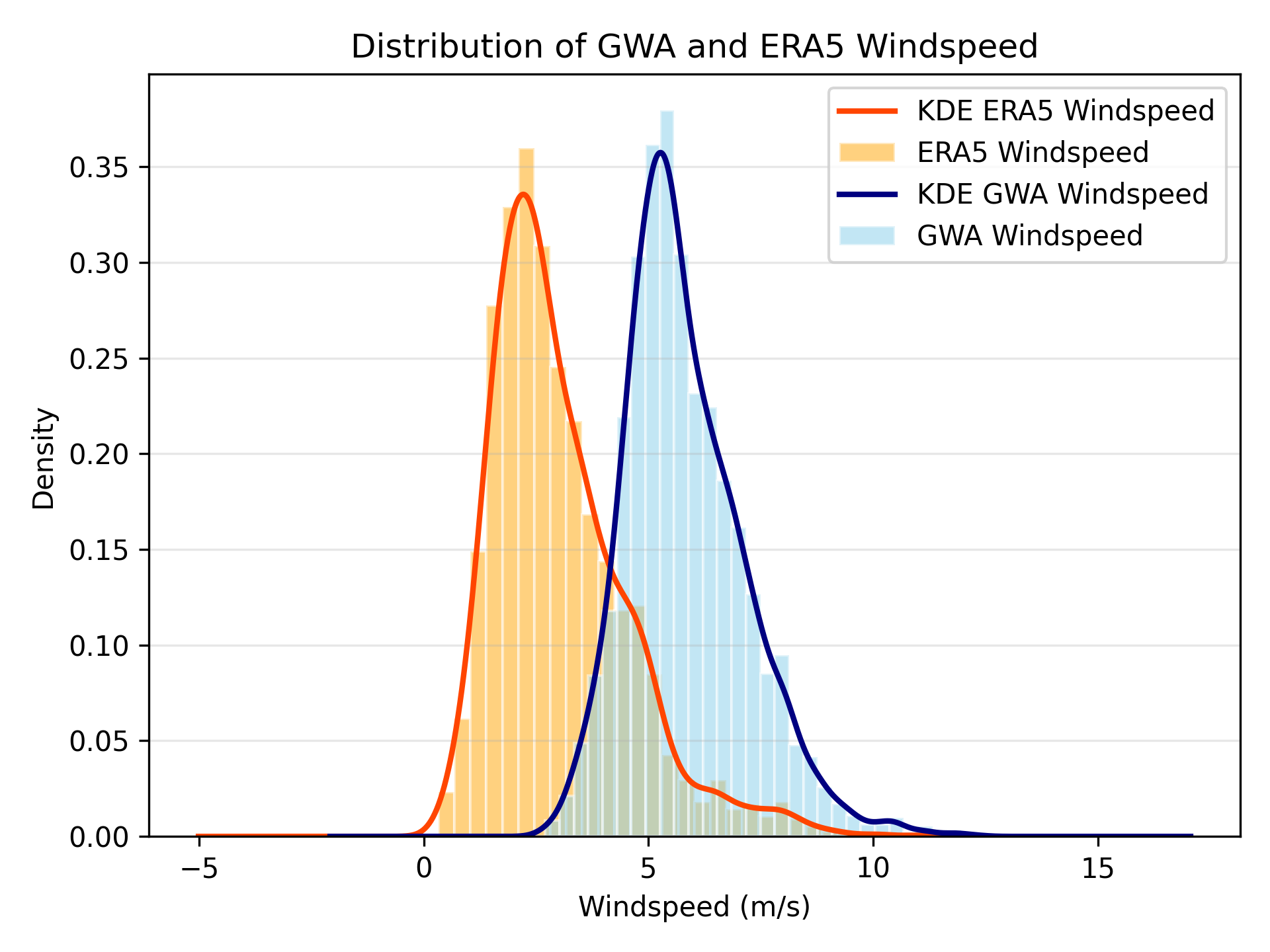
Here is a quick example from BC case study and how the rescaling looks like:
Attention
Working enhancement includes similar rescaling method for solar resources.
See also
extract_weather_data() , update_gwa_scaled_params() at RESource Builder.
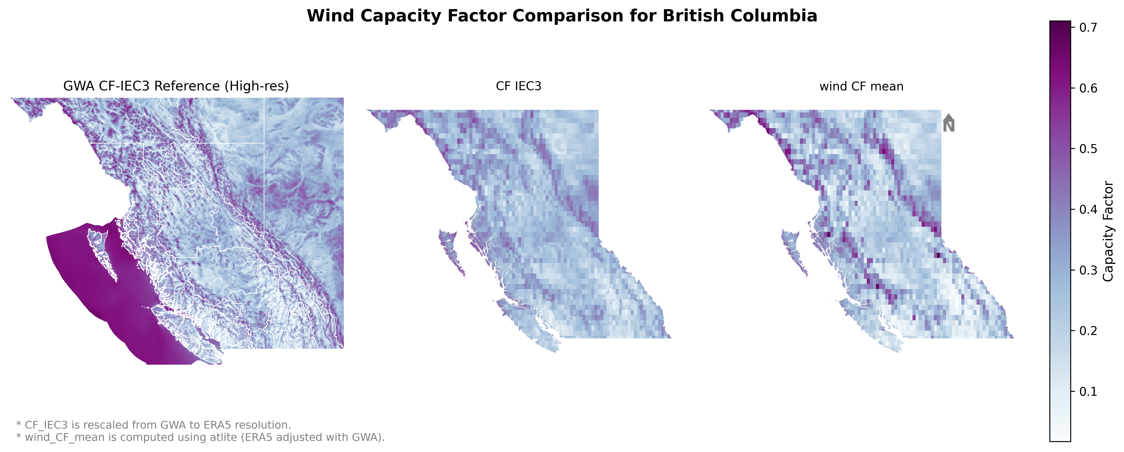
Extracts relevant weather data (e.g., wind speed, solar irradiance) for each grid cell. This calculation has been used for validation purposes. However, the available CF parameters (from different methods) could be used for scoring metric, energy calculations etc.
We compared CF for IEC Class 2,3 turbines sourced from GWA and compared with RESource's result CFs.
Updates grid cell parameters using Global Wind Atlas (GWA) data, scaling them as needed for accurate modeling.
Step 4: Get Timeseries#
See also
RES.timeseries.get_timeseries() at RESource Builder.
This method generates capacity factor (CF) time series for each grid cell using weather data and technology characteristics.
We define technology attributes.
We extract timeseries using weather resources data from ERA5's cutout.
The timeseries calculation method currently configured with atlite.cutout.pv and atlite.cutout.wind methods.
Attention
Configure the timezone conversion information carefully to ensure proper usage of the timeseries in downstream modelling.
ERA5 provides naive timezone index data. We use the timezone information from config file to enable the timezone shift of the timeseries.
However, after conversion we removed the timezone awareness from the datetime index to harmonize with pypsa supported timeseries index.
Tip
RES.timeseries.__fix_timezone__() method could be leveraged to reconfigure timezone awareness, if it is critical for your use-case of the timeseries.
Step 5: Find Grid Proximity#
This information is critical for downstream operational analysis with this resource options.
Attention
Currently configured for Transmission Lines and/or Grid Substations.
We do not know the specific project point of a resource. Hence, the resource to grid-node distance has been calculated from the centroid of each grid to the grid node.
If you have a specific project point, you should recalculate this distance with your specific project point.
Identifies and assigns grid nodes to each cell.
Calculates distance (in km) from each grid cell to the nearest grid node (e.g., transmission line, substation) to assess connectivity and feasibility for energy transport.
Tip
If your use case of the resource options are to be plugged in to a downstream operational model (e.g. PyPSA), use harmonized nodes to populate this data.
harmonized nodes i.e. same data that are intended to be used as bus nodes at your operational model.
See also
find_grid_nodes() at RESource Builder.
Step 6: Scoring Metric to Rank the Sites#
Attention
Currently scoring calculation is configured as simplified LCOE formula.
See also
RES.score.CellScorer.get_cell_score() at RESource Builder.
Scores each grid cell based on multiple criteria (e.g., resource quality, proximity to grid), supporting site selection.
relative cost scoring method (configurable)
\text{CRF} = \frac{r(1+r)^N}{(1+r)^N - 1}
CRF from discount rate (r) and life (N).
E_i = 8760 \times CF_i \times C_{\text{ref}}
Annual energy at site (i).
\text{Score}_i
= \frac{\text{CRF}\cdot C_i^{\text{cap}} + FOM_i + VOM_i \cdot E_i}{E_i}
\quad [\$/\text{MWh}]
Capital cost
C_i^{\text{cap}} = CAPEX_i \cdot C_{\text{ref}} + C_i^{\text{spur}} + C_i^{\text{upgrade}}
Grid costs are added on top of plant CAPEX; upgrades can be modeled as linear $/MW-km.
Symbols (units)
(r): discount rate; (N): project lifetime (yr).
(C_i_cap): total capital at site (i) using fixed (C_ref) (plant CAPEX + grid connection).
(FOM_i): annual fixed O&M at site (i).
(VOM_i): variable O&M ($/MWh).
(CF_i): capacity factor at site (i); (C_{\text{ref}}): fixed reference capacity (e.g., 100 MW).
Note: The score is a relative, LCOE-like screening metric (not investment-grade LCOE).
Hint
Working enhancement includes several scoring metrics to serve scenario analysis.
Future improvements are planned to include Multi-criteria Decision Analysis (MCDA) methods to make scoring more robust.
Step 7: Clusterized Representation of the Sites#
See also
get_clusters(), get_cluster_timeseries() at RESource Builder.
Groups grid cells into clusters based on spatial or resource characteristics to enable aggregated analysis.
Produces time series data for each cluster, summarizing the resource and capacity factor information at the cluster level.