Best Practices and Guidelines

Selecting Wind Turbines

IEC Class Selection

As recommended in The Global Atlas for Siting Parameters (GASP) project: Extreme wind,turbulence, and turbine classes, the parameter values applied at hub height 100m for different IEC classes are listed below. Suitability for a wind turbine depends on crucial factors like mean wind speed, turbulence, extreme wind speed, and air density in high winds. It is important to select the site-specific appropriate turbine class.

Wind Turbine Class	I	II	III
Vave (m/s)	10.0	8.5	7.5
Vref (m/s)	50.0	42.5	37.5
Vref,T (m/s)	57.0	57.0	57.0
A+ ref	0.18
A Iref	0.16
B Iref	0.14
C Iref	0.12

Table source: Table 1 from The Global Atlas for Siting Parameters (GASP) project: Extreme wind, turbulence, and turbine classes

Note: V_ave is the annual average wind speed; V_ref is the reference wind speed average over 10 min; V_ref,T is the reference wind speed average over 10 min applicable for areas subject to tropical cyclones. A+ designates the category for remarkably high turbulence characteristics; A for higher turbulence characteristics; B for medium turbulence characteristics; C for lower turbulence characteristics and I_ref is a reference value of the turbulence intensity.

IEC Class Layer Mapping to Select Turbine Technologies for Wind Energy Estimation

Layer Name	Wind Turbine Class Parameters
IEC Class - Fatigue Loads	Mean wind speed (Class I, II, III, S); Turbulence category (A+, A, B, C); Excludes wake effects
IEC Class - Fatigue Loads incl. Wake	Mean wind speed (Class I, II, III, S); Turbulence category (A+, A, B, C); Includes wake effects
IEC Class - Extreme Loads	Extreme wind speed; Air density at high wind speed (Class I, II, III, T, S)

Source: IEC Classes at GWA

This involves prioritizing the highest wind turbine class from the GWA's IEC Class layers prior to converting the wind resource potential to energy yield parameters. GWA includes three different IEC Class layers (under the Wind Energy Layers), mapping IEC wind turbine classes for 100m wind turbine hub height. Any wind turbine, regardless of its class, usually needs validation with the manufacturer specific to the site. GWA provides rasterized data to map wind turbine class recommendations for different load scenarios. For resource estimation studies, it is typically essential to evaluate the highest wind turbine class from the IEC Class layers in the GWA.

Best Practices

1. Layer Selection: Choose the most relevant GWA IEC Class layer (Fatigue Loads, Fatigue Loads incl. Wake, or Extreme Loads) based on your scenario/project’s objectives and local wind conditions.

   • Consider Wake Effects: For wind farm layouts, include wake effects in fatigue load assessments to ensure accurate turbine class selection.

   • Extreme Events: Factor in extreme wind events and air density when evaluating turbine class for long-term reliability.

2. From the layer, find the most appropriate IEC Class that represents most of your area of interest.

3. Documentation: Reference authoritative sources (e.g., GWA, IEC standards) and document all assumptions and data sources used in the selection process.

Example

For British Columbia (BC), the map on the right displays IEC turbine classes for the IEC Class - Extreme Loads layer. The analysis shows that IEC Class III turbines are most representative for this region under extreme load conditions. Areas marked in red indicates IEC Class II, likely due to significant terrain transitions such as mountainous slopes.

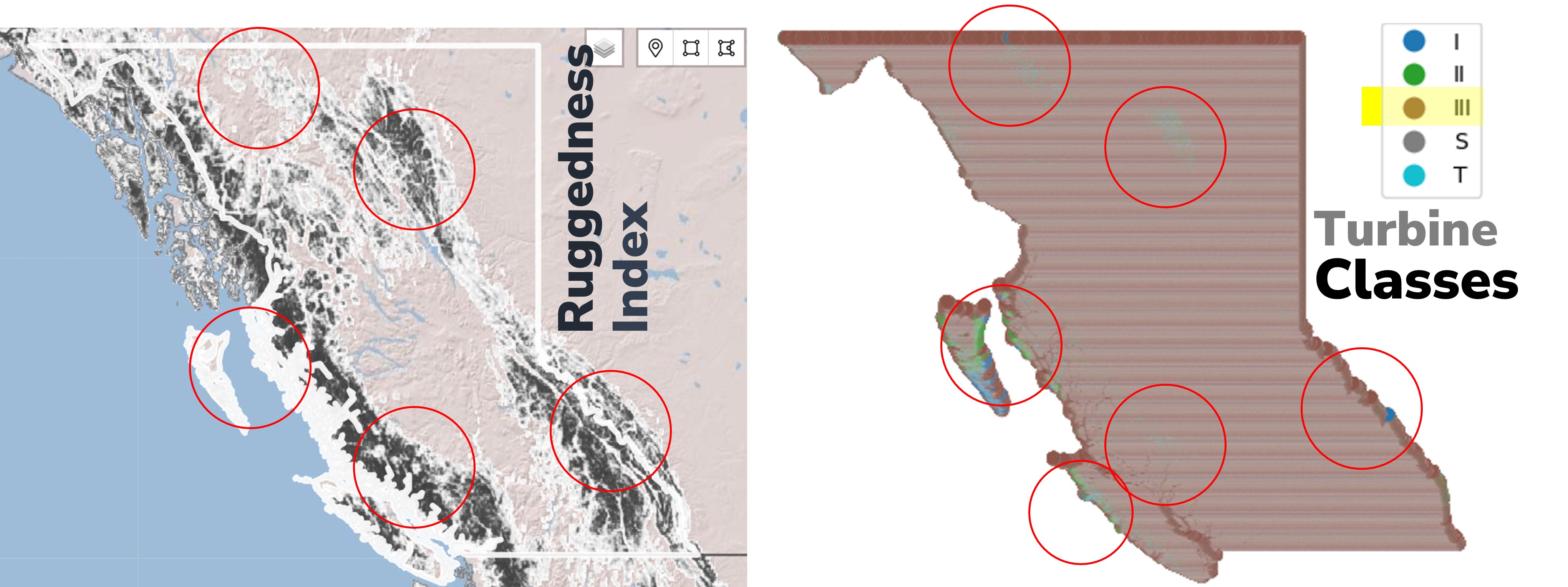
The Ruggedness Index (as shown in in left map), also known as the Terrain Ruggedness Index (TRI), quantitatively measures terrain heterogeneity by assessing elevation changes across the landscape. This index helps explain IEC Class variations in specific areas and supports informed decisions regarding IEC Class selection.

Data Source: Global Wind Atlas (GWA) _v3.4

Selecting Solar PV Panels

We use the atlite.pv conversion functionality to translate surface solar irradiance (direct + diffuse) and ambient temperature into photovoltaic (PV) power output. Internally, this module relies on a detailed panel model that incorporates parameters such as panel efficiency and temperature-dependent performance losses.

• Users can specify panel orientation (e.g., fixed tilt or azimuth) or tracking configurations (e.g., single-axis tracking). The “optimal” tilt—commonly based on latitude—or active tracking improves alignment with the sun, enhancing overall energy yield.

  For Optimal slope of the panels, atlite uses the formula documented in solarpaneltilt: Optimum Tilt of Solar Panels

• Currently, panel configuration options are limited to crystalline silicon (c-Si), cadmium telluride (CdTe), and Kaneka (amorphous silicon) technologies. The configurations and assumptions underlying the pv panel models can be found at atlite/resources/solarpanel

Panel Attribute Configurations:

• Higher-efficiency panels and improved orientation directly increase generation under identical irradiance conditions. If you do not want to explicitly define panel orientation, use tracking: 'dual' and we have defaulted the 'orientation': "latitude_optimal" at timeseries module.

  Examples regarding custom orientation configuration is provided here: atlite PV examples

• We configure the pv panels' attributes at 'capacity_disaggregation/solar' key of the config file.

Land Availability Calculation from Vector vs Raster Data

Vector and raster data are two fundamental ways of representing spatial information on computers. They each have their strengths and weaknesses, so the best choice depends on what you're trying to achieve.

Vector data is like a map made with geometric shapes. It uses points, lines, and polygons (areas) defined by mathematical coordinates to represent features. Imagine a map of a city with parks drawn as green polygons, streets as lines, and important buildings as points. This allows for sharp, clean lines and makes it easy to scale the map without losing quality. Vector data is also efficient for storing information about the features, like names, descriptions, or even photos.

Raster data, on the other hand, is like a photograph of the real world. It breaks down space into a grid of tiny squares, like pixels in a digital image. Each square holds a value that represents what's there, such as a color or an elevation level. Satellite imagery and scanned maps are common examples of raster data. Raster data excels at capturing continuous variation and is often simpler to process for certain analyses. However, it can become bulky for large areas and lose detail when zoomed in.

Here's a table summarizing the key differences:

Feature	Vector Data	Raster Data
Representation	Points, lines, and polygons	Grid of squares (pixels)
Detail at high zoom	Crisp and clear	Can appear blocky or pixelated
Scalability	Excellent, maintains quality when zoomed	Loses detail when zoomed in
File size	Smaller for similar detail	Larger for continuous variation
Feature information	Can store additional data about features	Limited to data represented by pixel values
Common uses	Maps, logos, illustrations	Satellite imagery, photographs, elevation data

Ultimately, the choice between vector and raster data depends on analysis specific needs. If you need precise shapes and sharp lines, vector data is the way to go. But if you're working with continuous data or imagery, raster data might be a better fit.

Open Street Map (OSM) Data

Goal:

• To create vector data with targeted landuse. e.g. we have used 'aeroway' vector data in this analysis.

What is 'aeroway'?

Usage in RESource (Linking Tool):

• 1. We can filter the type of aeroway landuse that we want to disregard as a potential site.

• 2. We will create a union geometry of all aeroway area, and later can add buffer area around surrounding this geometry. The Buffer radius can be configured via the user configuration file.

• 3. We will exclude this final geometry [aeroway union+buffer] from our Cutout Grid Cells during land availability calculations for potential VRE sites.

Tool :

We used pyrosm to extract OSM data via python API.

why pyrosm?

Method:

• We created an OSM 'object' which has various attributes. One of the attributes is 'point of interests (get_pois)'.

• Each attribute has several 'keys'. We used 'get_pois' method to extract one of the available 'keys' (e.g. 'aeroway')

• Each OSM key has several tags associated e.g.

from pyrosm.config import Conf
print("All available OSM keys", Conf.tags.available)
print("\n")
print("Typical tags associated with Aeroway:", Conf.tags.aeroway)

All available OSM keys ['aerialway', 'aeroway', 'amenity', 'boundary', 'building', 'craft', 'emergency', 'geological', 'highway', 'historic', 'landuse', 'leisure', 'natural', 'office', 'power', 'public_transport', 'railway', 'route', 'place', 'shop', 'tourism', 'waterway']

Typical tags associated with Aeroway: ['aerodrome', 'aeroway', 'apron', 'control_tower', 'control_center', 'gate', 'hangar', 'helipad', 'heliport', 'navigationaid', 'beacon', 'runway', 'taxilane', 'taxiway', 'terminal', 'windsock', 'highway_strip']

• We used custom filters to extract data for our target key 'aeroway'

How to read and visualize Point of Interests? How to custom filter OSM data

Why subnational dissolved polygons were used instead of a single country boundary

Core issue

In the earlier workflow, boundary cells at the national edge could be unintentionally double counted or misallocated when an ERA5 cell intersected multiple geometries. This happened because the availability and capacity calculations were first performed at the country-dissolved ERA5-cell level, and only afterward the trimmed cell was overlaid with smaller internal geometries.

A critical distinction is that the final “sites” in this workflow are not the ERA5 cells themselves. Rather, the sites are the geometries inside the ERA5 cells, which emerge after applying higher-resolution raster and vector constraints. These internal geometries are therefore the planning-relevant units for capacity allocation.

Why a single country boundary was not sufficient

Using a single dissolved country boundary is adequate for national masking, but it is not adequate for intra-national attribution. It only answers whether a cell lies inside the country, not how capacity should be distributed across subnational units within that cell.

To preserve intra-national spatial resolution, polygons dissolved by subnational administrative units were used instead of a single country geometry. This allows each resulting geometry to be assigned to a planning-relevant administrative region, enabling region-wise aggregation of:

• land availability,

• capacity potential,

• and cost metrics such as LCOE.

In contrast, a single country polygon removes the internal regional structure that is needed for subnational energy planning and municipal or regional investment prioritization.

Example

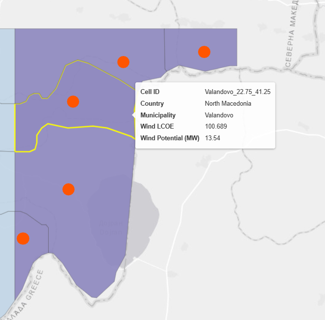
Interpretation The purple polygon shows a single ERA5 cell after trimming to the country or regional boundary. The five internal polygons correspond to municipality-level geometries located inside that same trimmed ERA5 cell. Since these polygons are subdivisions of one parent ERA5 cell, they initially share the same underlying cell-level attributes. This example highlights the distinction between the meteorological grid cell and the planning-relevant administrative geometries embedded within it.

The earlier workflow was:

1. pass the country-dissolved geometry into the availability matrix,

2. calculate the capacity matrix,

3. derive capacity at the ERA5-cell level,

4. then overlay the trimmed ERA5 cell with municipality geometries.

The problem with this sequence is that each municipality geometry could end up absorbing the same cell-level capacity, even though those geometries may differ strongly in their actual developable land. In other words, the boundary trimming created multiple internal geometries, but the capacity signal was still inherited from the undifferentiated ERA5 cell.

Two possible correction methods

Method A: Area-proportional scaling

One correction is to assume that land availability within the ERA5 cell is uniformly distributed across all internal geometries. Under that assumption, municipal capacity can be scaled as:

municipal capacity = ERA5-cell availability × municipality geometry area

This is simple and internally consistent if no better spatial information exists. However, it assumes that developable land is spread evenly within the ERA5 cell. Where municipalities differ strongly in land cover, slope, protected areas, buffers, or other siting constraints, this can become spatially misleading. It may allocate too much capacity to municipalities with little suitable land and too little to those with more developable land.

Method B: Geometry-level availability breakdown

The second correction is to calculate availability at the municipality-geometry level, rather than only at the ERA5-cell level. In this case, each internal geometry receives its own availability estimate derived from the finer-resolution spatial data. Capacity is then calculated from that geometry-specific availability.

This approach preserves the true spatial heterogeneity of developable land within a single ERA5 cell and avoids the artificial assumption of uniform distribution.

Method applied here

Method B was applied.

This is preferable because the workflow already uses high-resolution spatial inputs, including raster and vector constraints, to determine land availability. Since those data capture internal differences within the ERA5 cell, capacity allocation should also reflect those differences.

This makes the results more spatially defensible, especially when municipalities within the same ERA5 cell differ substantially in their actual developable land.

Why this is justified with 100 m data

The use of high-resolution data is important here. Availability was derived using 100 m raster information together with vector exclusions/constraints, so the workflow is not relying on coarse cell-wide assumptions alone. If a municipality geometry contains many 100 m pixels, then its developable fraction is meaningfully estimated from actual spatial detail rather than from a uniform average.

This means the geometry-level availability values are not arbitrary subdivisions of the ERA5 cell. They are grounded in the spatial pattern of:

• land cover,

• exclusion zones,

• protected areas,

• buffers,

• and other vector/raster siting constraints.

As a result, geometry-level capacity estimates are relevant for municipal or subregional interpretation, provided the geometry is large enough to be represented meaningfully at the 100 m resolution.

Role of raster and vector data in atlite availability calculations

In atlite, availability is typically computed by evaluating which parts of a grid cell remain suitable after applying exclusion layers. In this workflow, that logic is enriched by combining:

• high-resolution raster layers (for example land cover or gridded suitability data), and

• vector layers (for example administrative boundaries, protected areas, lakes, buffers, or other exclusion geometries).

Conceptually, the process is:

1. start from the coarse ERA5 grid cell,

2. evaluate suitability inside that cell using fine-resolution raster data,

3. exclude or trim unsuitable portions using vector constraints,

4. retain only the eligible land fragments,

5. aggregate those eligible fragments into geometry-level availability values.

Because of this raster–vector combination, the final “site” is better interpreted as a reality-corrected developable geometry inside an ERA5 cell, not as the ERA5 cell itself.

Why this matters even if capacities are later aggregated

Even if the final model aggregates all municipal geometries into a single resource or supply option, the spatial breakdown remains valuable.

It helps answer questions such as:

• where the aggregated capacity is actually located,

• which municipalities or subregions contribute most,

• whether investment potential is spatially concentrated or dispersed,

• and which areas may deserve prioritization for planning, infrastructure, or permitting.

So although the optimization model may later collapse these sites into a larger resource class, the finer spatial decomposition still provides important planning intelligence. It supports interpretation, transparency, and investment prioritization in ways that a single aggregated number cannot.

The key methodological shift was moving from country-level ERA5-cell capacity allocation to subnational geometry-level availability and capacity allocation. This avoided misallocation at boundaries, preserved intra-national spatial structure, and better reflected the true distribution of developable land captured by the 100 m raster and vector exclusion workflow.

In short:

• a single country boundary is sufficient for national masking,

• but subnational dissolved polygons plus geometry-level availability are needed for spatially just and planning-relevant capacity allocation.